Appendix F: The Overstated Earnings Hypothesis in Accounting Simulation

In this appendix, we're going to walk through an accounting simulation that illustrates how an illusory profitability gap can emerge entirely from inflation-related inaccuracies associated with historical cost accounting. To allow readers to follow along with the simulation and experiment with it, we link to a spreadsheet containing the simulation below: 

• Accounting Simulation Spreadsheet

Strategy for the Simulation: Four Phases

The simulation will proceed in four phases: 

Phase I: Actual Real Values - In the first phase, we're going to construct a perfectly efficient hypothetical index with a cost of equity, a return on equity and a real fundamental return that are always equal to the real fundamental return observed in the S&P 500. We're also going to assume that the hypothetical index's depreciation rate and real interest rate match the average rates observed in the S&P 500. Assuming an environment of zero inflation, we're then going to compute the actual real financial quantities (assets, debt, equity, share price, EBIDA, depreciation, interest, earnings, dividends, etc.) that the hypothetical index ends up producing and accumulating over time. Note that these numbers will reflect the index's true quantities, expressed in real terms. 

Phase II: Actual Nominal Values - In the second phase, we're going to upwardly-adjust the real numbers computed in Phase I to reflect what the underlying quantities would come out to if expressed in terms of a price index that is inflating at a certain specified rate. Note that these numbers will reflect the index's true quantities, expressed in nominal terms. 

Phase III: Calculated Nominal Values - In the third phase, we're going to recalculate the nominal asset values, equity values, depreciation expenses and earnings in Phase II using historical cost accounting rules. Note that these nominal numbers will be distorted by the accounting framework and will not reflect actual true nominal quantities for the index. The earnings, in particular, will become overstated over time, laying the seeds for a profitability gap.

Phase IV: Calculated Real Values - In the fourth phase, we're going to apply the integrated equity methodology to the calculated nominal values in Phase III to calculate real values for the hypothetical index. Note that these real numbers will carry forward the distortions in Phase III and will not reflect actual true quantities for the index. Relative to the actual real values observed in Phase I, the index's cost of equity will show up as significantly overstated and its return on equity will show up as significantly understated, creating an illusory profitability gap. 

The goal of the simulation will be to demonstrate that when we set the parameters of the hypothetical index to match the actual average parameters observed in the S&P 500 from 1964 to 2018, and we then apply historical cost accounting rules to calculate the earnings and equity values of the hypothetical index over time, the illusory numbers that we calculate end up closely matching the actual average reported numbers that we see in the S&P 500 over the period, suggesting that those numbers, and the profitability gap that they give rise to, are illusory as well. 

Constructing the Simulation

If the S&P 500 were perfectly efficient, its cost of equity and return on equity would both be equal to its fundamental return at all times. For the 1964 to 2018 period, that return averaged out to 5.48%. Since the purpose of our hypothetical index is to represent a perfectly efficient version of the S&P 500, we're going to set its cost of equity, return on equity and fundamental return to be equal to 5.48% as well. Necessarily, an index with a cost of equity and a return on equity that are always the same will trade at a true P/IE ratio of 1.0.

In an effort to further mimic the S&P 500, we're going to set additional parameters for the hypothetical index as follows:

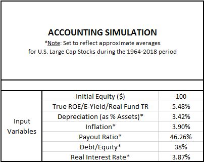
The depreciation¹, inflation, payout ratio, debt-to-equity² and real interest rate³ parameters are each chosen to match the actual average parameters observed in the U.S. Large Cap Stock Universe during the 1964 to 2018 period. 

Phase I: Actual Real Values

In Phase I, we calculate actual real values for the hypothetical index under the perfect efficiency assumption specified above. We start the index out in 1964 and allow it to generate earnings based on its characteristics:

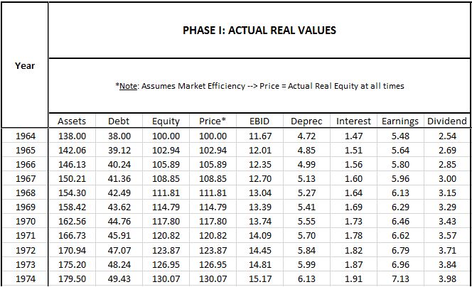
Note that all of these terms are real terms. The price index is not changing in this phase of the simulation. 

Initial Values: 1964

Here are descriptions of how each initial 1964 term is calculated, listed in the order in which it is calculated: 

• Equity: The index starts out with $100 in equity.
• Price: Per the efficiency condition, price must always equal equity, so price equals $100.
• Debt: The debt-to-equity ratio is set at 38%, so debt is $38.00 (=$100 * 38%).
• Assets: Assets equal debt plus equity, which is $138.00 (=$100 + $38).
• Earnings: Earnings are set at 5.48% of equity, therefore $5.48 (=$100 * 5.48%). 
• Depreciation (Deprec): Depreciation is set at 3.42% of total assets (corresponding to an approximate 29 yr average useful life for the overall balance sheet), so the depreciation expense comes out to $4.72 (=$138 * 38%).
• Interest: The real interest rate is set at 3.87% of debt. We arrive at this assigned number by taking the average nominal corporate interest rate for the period, 7.77%, and subtracting the average inflation rate, 3.90%. By subtracting inflation from the measure, we capture the real gain that accrues to the index when a portion of its debt is inflated away each year.
• EBID: To calculate EBID, i.e., earnings before interest and depreciation, we simply add interest and depreciation back to earnings. We get $11.67 (=$1.47 + $4.72 + $5.48)
• Dividend: The dividend is a value that is unknown to us in this phase of the simulation. The company will pay dividends based on what it thinks its nominal earning are, and we don't know what that number is yet. We're going to find out what it is when we get to Phase III, the section where we use GAAP rules to calculate nominal earnings. For 1964, the calculated number will end up being $2.54. 

Subsequent Values: 1965 and Onward

The terms for subsequent years are calculated in the same way as above. The two exceptions are equity and debt: 

• Equity: To calculate the subsequent equity of the index, we add the prior year's retained earnings to the prior year's equity--in other words, the prior year's equity, plus the prior year's earnings, minus the prior year's dividend. For 1965, that comes out to $102.94 (= $100 + $5.48 - 2.54).
• Debt: To calculate the index's subsequent debt, we assume that the index intentionally increases (or decreases) its real debt in all periods to maintain a constant 38% debt-to-equity ratio. For 1965, that means it increases its debt by $1.12 to $39.12. 

Assets, which are equal to debt plus equity, reflect the increases in both terms. For 1965, the asset total comes out to $142.06 (= $138.00 + $5.48 - $2.54 + 1.12). As explained elsewhere in the piece, we assume that the difference between cash earnings (EBID, which equals $11.08) and actual earnings ($5.48) is used to refurbish the previously-existing asset base, counteracting its depreciation and allowing us to continue to carry it at the same value that it had in the prior period, in this case $138.00.

Phase II: Actual Nominal Values

In Phase II, we set up a consumer price index (CPI) and steadily increase it over time to match the specified inflation rate for the simulation, 3.90%. We then upwardly-adjust the real values in Phase I to accurately express them in terms of the increasing price index.

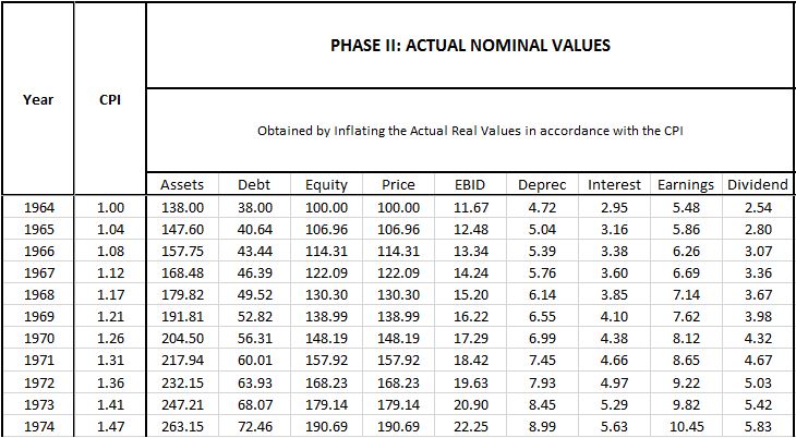
The only value that is not calculated in this way is nominal interest. We calculate it by multiplying the nominal interest rate (i.e., the real interest rate plus the inflation rate) by the nominal amount of debt. For 1964, that number comes out to $2.95 (= 7.77% * $38).

Phase III - Calculated Nominal Values

In Phase III, we calculate nominal values for the index under a historical cost accounting framework. 

Conceptually, we can separate the values in the simulation into those that that are determined through direct measurements and those that are determined through the application of historical cost accounting rules:

• Determined through Direct Measurement: Debt, Price, EBID, Interest, Dividends.
• Determined IAW Historical Accounting Rules: Assets, Equity, Depreciation, Earnings. 

For directly-measurable quantities, the calculated nominal values in Phase III are identical to the actual nominal values in Phase II. The accounting paradigm cannot introduce errors into these values because they're not determined through the application of accounting rules; rather, they're determined by simply looking at the quantities themselves, which are empirical and verifiable. 

For quantities that are determined through the application of historical cost accounting rules, the values in Phase III will be different from Phase II because the values in Phase III will not have been properly adjusted to reflect the changing price index.

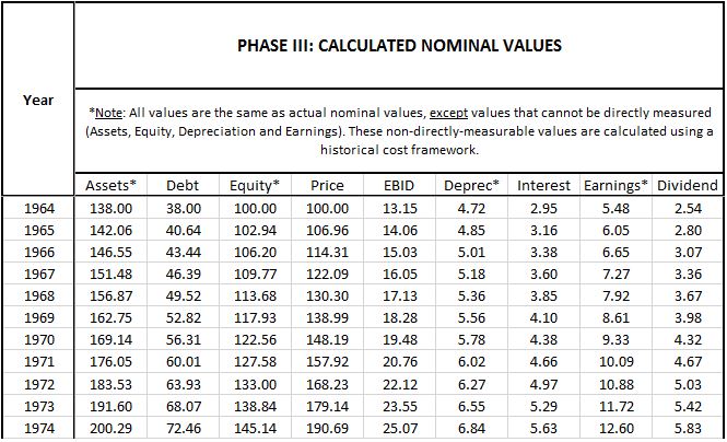
Here is a description of how each nominal term is calculated: 

• Debt, Price, EBID, Interest: Because these values are directly measurable, they are the same as in Phase II. 
• Equity: For 1964, the index's nominal equity is the initial equity value, $100. To calculate the nominal equity for subsequent years, we increase the prior year's nominal equity by the prior year's nominal retained earnings. For 1965, the total comes out to $102.94 (= $100 + $5.48 - $2.54). The source of the discrepancy between the value in Phase II ($106.96) and the value in Phase III ($102.94) is that the value in Phase II is derived from terms that are upwardly-adjusted to reflect the increased price index, whereas the value in Phase III is derived from terms that are being carried at unadjusted historical cost. Consequently, the Phase III value understates the actual true nominal equity.
• Assets: To calculate the nominal value of the index's assets, we add the equity value to the debt. For 1965, the result comes out to $142.06 (= $102.94 + $40.64). The nominal assets end up being understated because the nominal equity is being understated. 
• Depreciation: To calculate the nominal depreciation, we multiply the nominal value of the assets by the depreciation rate. For 1965, the number comes out to $4.85 (= $142.06 * 3.42%). This expense is understated relative to the actual nominal expense calculated in Phase II ($5.04) because the $142.06 asset value that it's calculated from is understated at historical cost. 
• Earnings: To calculate the nominal earnings, we subtract interest and depreciation from EBID. For 1965, the number comes out to $6.05 (=$13.43 - $4.85 - $2.53). This number is overstated relative to the actual nominal earnings in Phase II ($5.86) because the depreciation expense is being understated. 
• Dividend: We calculate the dividend by multiplying the calculated nominal earnings (which is what the company thinks its earnings are) by the payout ratio. For 1965, the number comes out to $2.80 (=$6.05 * 46.26%). (Note: this term is the official true dividend for the entire simulation and feeds back to the stated dividend values in all of the other phases, adjusted for inflation where applicable.) 

Phase IV - Calculated Real Values

In Phase IV, we calculate real values for the index by applying the integrated equity methodology to the calculated nominal values in Phase III:

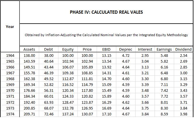
The only terms that end up being important here are the calculated real earnings and the calculated real equity: 

• Earnings: The calculated real earnings are obtained by inflation-adjusting the calculated nominal earnings in Phase III back down to 1964 prices. For 1965, the calculated real earnings number comes out to $5.82 (= $6.05 * 1.000 / 1.039). This number is overstated relative to the actual real earnings number observed in Phase I ($5.64) because it's derived from the overstated nominal earnings number calculated in Phase III. 
• Equity: The calculated real equity in each year is equal to the prior year's calculated real equity plus the prior year's calculated real retained earnings (i.e., calculated real earnings minus the real dividend). For 1966, the first year where a discrepancy emerges relative to Phase I, the calculated real equity comes out to $106.07 (=$102.94 + $5.82 - $2.69). This number is overstated relative to the actual true $105.89 number observed in Phase I because it's based on a 1965 earnings term that is overstated. 

Calculating Metrics for the Index

Using values from the four phases of the simulation, we can calculate relevant metrics for the hypothetical index and observe their trajectories over time. We separate the metrics into reported, actual and integrated. 

• The "reported" metrics--e.g., reported valuation (P/B ratio), reported cost of equity (reported earnings yield, or reported earnings divided by price) and reported return on equity (conventional inflation-unadjusted ROE, or reported earnings divided by reported equity)--are derived from the calculated nominal values in Phase III. Note that these values are incorrect. They've been artificially inflated by the overstatement of earnings and the understatement of equity. 
• The "actual" metrics--e.g., actual valuation (price-to-equity ratio), cost of equity (earnings yield, or earnings divided by price) and return on equity (earnings divided by equity) are derived from the actual true numbers in Phase I and Phase II. Note that these metrics are the correct, true metrics for the index. Since they're ratios, we can use either Phase to calculate them, as long as we're consistent. 
• The "integrated equity" metrics for the index--e.g., valuation (price-to-integrated equity ratio) and return on equity (current real earnings divided by initial real equity plus the sum of calculated real retained earnings)--are derived from calculated real values in Phase IV. These metrics are the metrics that we calculated in the piece using the methodology. As explained above, they're incorrect because they're derived from retained earnings and equity measurements that are overstated. 

The chart below shows the trajectories of relevant metrics over time in the simulation:

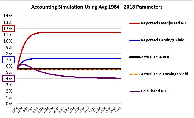
All of the metrics start out at 5.48%, which is the actual true value of all of the quantities that the metrics are seeking to represent. As inflation builds, the reported metrics and the metrics calculated in accordance with the integrated equity methodology deviate from that value: 

• Reported Unadjusted ROE (red): The reported ROE, which is unadjusted for inflation, rises dramatically. Its numerator, earnings, becomes overstated, while its denominator, equity, becomes understated. The result ends up being a gross overstatement in the overall expression. Interestingly, the number that the ROE equilibrates at, 11.40%, is exactly equal to the reported nominal earnings growth rate (~6.127%) divided by the reported retention rate (i.e., one minus the 46.26% reported payout ratio, i.e., 53.74%), consistent with the formula that we derived in Appendix A, Claim #5. 
• Reported Earnings Yield (blue): The reported earnings yield rises as the earnings become overstated.
• Calculated ROIE (purple): The calculated return on integrated equity falls. In the presence of overstated earnings, the sum of real retained earnings becomes overstated, causing the equity term in the denominator to become overstated. Because this sum is cumulative, it eventually becomes more overstated than the earnings term in the numerator, causing the overall ROIE expression to become understated. The point of inflection, where the overstatement in the denominator ends up exceeding the overstatement in the numerator, with the expression turning downward, happens approximately ten years into the simulation. Interestingly, the return on differential equity (RODE) measurement, which is described in Appendix B, equilibrates at the same value as the ROIE, confirming that it's a valid long-term proxy for the ROIE. 

Given that the reported earnings yield equilibrates at a value (7.21%) that's significantly higher than the calculated ROIE (3.99%), the index ends up with a large profitability gap (3.22%). 

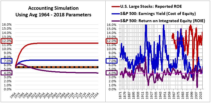
Inferring the Primary Cause of the S&P 500's Profitability Gap

The simulation confirms what we already knew, which is that a perfectly-efficient index can develop an illusory profitability gap entirely from distortions associated with historical cost accounting. What we didn't know, and what we still don't know, is how much of the S&P 500's actual profitability gap is due to those distortions. 

Recall that we set the environmental and operational parameters of the simulated index to be equal to the actual average parameters observed in the S&P 500 from 1964 to 2018. By comparing (1) the illusory profitability gap that emerges at equilibrium in the simulation due to flawed accounting and (2) the actual profitability gap seen in the actual S&P 500 over the period, we can estimate the relative contribution that accounting distortions are making to the actual gap. 

The juxtaposed chart below facilitates the comparison. When we compare the differences between the blue line and the purple line in the simulation and the actual S&P 500, we see similar numbers for the lines (approximately 7% and 4%, respectively) and a similar gap between them (approximately 3%):

In the table below, we compare the metrics calculated in the simulation at equilibrium to the actual average calculated metrics for the S&P 500 over the period:

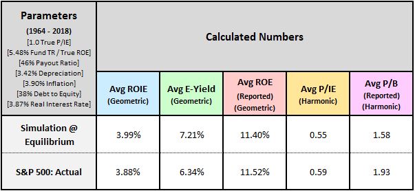
As you can see, the metrics match each other very closely. We discuss each metric below: 

• Avg ROIE: The equilibrium calculated ROIE in the simulation comes out to 3.99%, only 0.11% off from the ROIE calculated for the actual S&P 500. 
• Avg E-Yield: The equilibrium average earnings yield in the simulation comes out to 7.21%, 0.87% higher than the 6.34% average earnings yield calculated for the actual S&P 500. The difference is noticeable, but we have to remember that the simulation assumes that the index always trades at fair value, with an actual true P/IE ratio of 1.0. This assumption does not apply to the actual S&P 500, which spent more time above fair value than below it during the 1964 to 2018 period. We should therefore expect the S&P 500's actual average earnings yield to be slightly depressed relative to the equilibrium earnings yield in our simulation, which is precisely what we see in the data.
• Avg Reported ROE: The average reported ROEs come out almost exactly the same, separated by only 0.12%.
• Avg P/IE: The average P/IE ratios come out roughly the same, separated by a difference of roughly 8%. The valuation point made above applies here. We should not be surprised that there's a difference between the average measured valuations of the index in the simulation and the index in reality. Unlike the index in the simulation, the actual index in reality traded at an average above fair value during the period. 
• Avg P/B: The average P/B ratios come out roughly 30% apart, a fact that can again be explained by the actual index's greater expensiveness over the period.

The fact that the metrics line up so closely is strong evidence that the majority of the profitability gap observed in the actual S&P 500 is due to inflation-related earnings overstatement associated with the use of a historical cost framework. It's possible, and likely, that earnings have been overstated across history in other ways and for other reasons, but the historical cost reason is likely the main reason. 

Estimating the Severity of Earnings Overstatement as a Function of Inflation

At equilibrium, the degree of earnings overstatement that emerges in the simulation is 32%. This number is associated with an inflation rate of 3.90%. By running the simulation at other rates of inflation, we can build a mapping between the inflation rate and the severity of earnings overstatement more generally. When comparing valuations across different periods of history, we can then use the mapping to correct for relevant differences in inflation.

In the table below, we show the degree of overstatement that emerges in the simulation under inflation rates ranging from 0% to 10%:

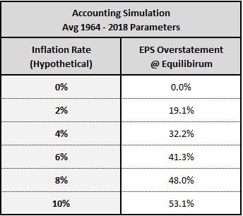
In the piece, we estimated the average degree of earnings overstatement across the 1871 to 2018 period by searching for the degree of overstatement that, if reversed, would create the closest match between the average cost of equity and the average return on equity. We eventually arrived at an estimated degree of overstatement of 25%. We can corroborate this estimate using the table above by noting that inflation over the 1871 to 2018 period was 2.07%. That number corresponds to an estimated degree of overstatement of approximately 20%, not far from our earlier 25% estimate.

Whitepaper Links

• The Earnings Mirage: Why Corporate Profits are Overstated and What It Means for Investors.
• Appendix A: An Intuitive Example that Clarifies Important Claims Made in the Piece
• Appendix B: Calculating the Return on Differential Equity
• Appendix C: Solving for Initial Equity
• Appendix D: The Payout Ratio Method
• Appendix E: Integrated Equity Data for Sectors, Industries, Countries and Factors
• Appendix F: The Overstated Earnings Hypothesis in Accounting Simulation
• Appendix G: Initial Equity in the PIE Ratio Calculation

Footnotes

¹ This term also includes the depletion of natural resources and the amortization of intangible assets.

² The average debt-to-equity ratio for the period is calculated using nonfinancial corporate debt in the numerator and nonfinancial corporate net worth at market value in the denominator, both of which are obtained from the flow of funds report (Z.1, B.103). Reported company equity cannot be used in the calculation of debt-to-equity because it is carried at historical cost and is therefore severely understated relative to reality. 

³ The real interest rate is calculated as the average of Moody's seasoned AAA and BAA bond yields minus the inflation rate.