Appendix B: Calculating the Return on Differential Equity
By Jesse Livermore+
July 2019
In this appendix, I'm going to introduce a technique for measuring the incremental ROE of a company or index over a given period. This technique will be used in Appendix B to solve the initial equity problem.
To frame the technique, let's imagine investing as an activity in which we use cash to build machines that spit out cash. Suppose that I start out in December 1968 already owning a cash machine that spits out $1 per year. We don't know how much I paid to build or acquire this machine, so we don't know what the machine's ROE is. But we know what it spits out each year--$1.
Suppose further that I take 100% of the cash proceeds of this machine and use them to build new machines that spit out cash. In the same way, I reinvest the proceeds of those new machines, building even more new machines, and so on in a compounding process. At the end of the process, I end up with a collection of machines--the original machine plus the new ones that I built--that are now producing a total of $23 per share.
Let's assume that the total amount of money that I reinvested into the new machines over the period was $371 dollars. The question that we want to answer is, given these numbers, what is the implied ROE on the new machines?

We can solve for the answer using simple math. We know that the original machine produces $1 per year. We also know that the final collection of machines, which includes the original machine and all the new machines, produces $23 per year. It follows that the new machines produce the difference, $22 per year. We know how much those machines cost--$371 in total, which is the full amount that was reinvested over the period. It follows that the ROE on the new machines--the cash flow stream they spit out divided the amount of cash that went into building them--is $22 /$371, or roughly 6%.
I'm going to refer to this 6% value as the return on differential equity, or "RODE". The RODE over a specified period is given by the following equation. Note that all numbers must be inflation-adjusted:
RODE = Change in EPS / Sum of Retained EPS
When we calculate the RODE, we're taking the earnings added by an interim investment process--i.e., the difference between the earnings at the beginning of the process and the end of the process--and dividing those earnings by the total amount of money that went into the process. In this way, we're calculating the return on the differential equity that was added by the process, hence the name.
Crucially, to calculate the RODE for an investment process, we don't need to know the equity or book value at the beginning or the end of the process. All we need to know is the intervening change in equity that occurred during the process, i.e., the total intervening investment that took place within it.
The following chart shows $CAT's RODE for periods starting in 1964 and ending on subsequent dates ranging from 1965 through 2018:
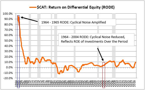
Notice that $CAT's RODE for the one-year period from 1964 through 1965 was extremely high--on the order of around 95%. That's because the change in its earnings over that year (the numerator in the RODE) was very large relative to the amount that it reinvested over the year (the denominator in the RODE). But the change in its earnings over the year was not caused by any of the investments that it made during the year. Rather, the change was caused by cyclical fluctuations in the company's business. Consequently, the company's RODE for the 1964 to 1995 period doesn't provide any useful information on its incremental ROE during that period.
As the ending boundary of the RODE calculation is increased from 1965 to later dates, the RODE numbers become significantly more informative. The denominator of the metric gets larger, reducing the amplification of short-term noise. The numbers then begin to track with the actual returns that the company's intervening investments are producing. We see this effect, for example, in the 2004 data point. It represents the change in earnings from 1964 to 2004 divided by the change in equity. There's still cyclicality in the number, because we're comparing earnings on two individual dates in history, but the cyclicality isn't amplified to the same extent. The overall ratio ends up being driven primarily by the underlying ROE of the investments that were added during the period, bringing it to a more sensible level, roughly 5%.
When calculated across an extended period of time, the RODE provides a reasonably accurate measurement of a company's incremental ROE. In Appendix B, we explain how to use long-term RODE data to back-calculate initial equity values and solve the initial equity problem.
Whitepaper Links