Appendix C: Solving for Initial Equity
By Jesse Livermore+
July 2019
In this appendix, I'm going to explain how we can use the return on differential equity (RODE) measure described in Appendix A to solve the initial equity problem.
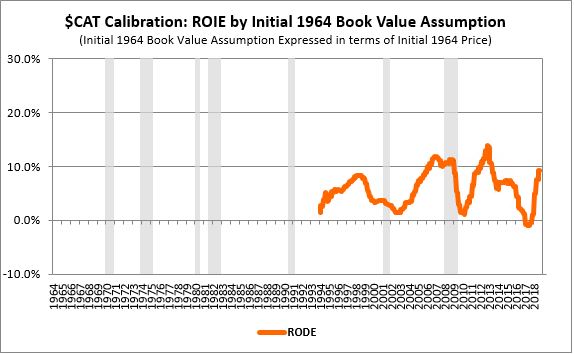
The process is best explained in terms of our earlier example of Caterpillar ($CAT). We start by calculating $CAT's RODE for periods beginning in 1964 and ending on dates ranging from 1993 through 2018. We choose these distant years as the end dates for the calculations because we want to minimize the amplification of cyclical noise in the RODE measure. We then plot the results for each ending date:
That's the first step. In the second step, we assume an arbitrary number for the unknown 1964 equity value and compute a subsequent time series of integrated equity values based on that starting number. We then divide the real EPS on each date by the associated integrated equity values that we calculate, obtaining a time series of the return on integrated equity (ROIE).
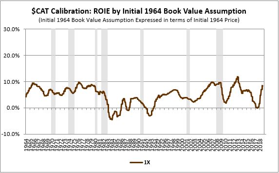
The chart below provides an example of one way of completing the second step. We arbitrarily assume that the company's inflation-adjusted equity value in 1964 was exactly equal to its inflation-adjusted price on that date. We then add the company's subsequent history of real retained EPS to that starting value to obtain future integrated equity values. Finally, we divide the real EPS on each date by those values, obtaining the ROIE series shown below:
In the third step, we put these two series together on the same chart and compare them. We calculate the square difference between the lines and use that as an approximation for the accuracy of our initial 1964 equity assumption:
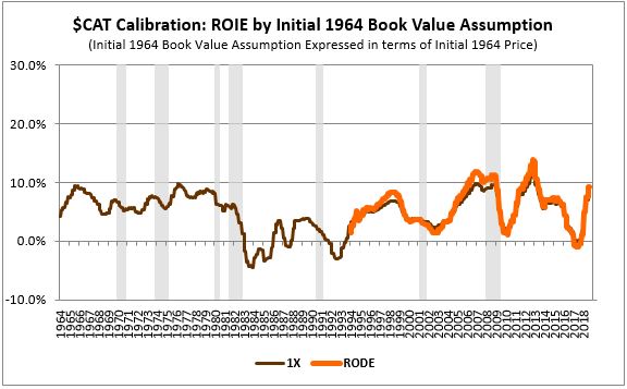
As expected, the ROIE measure (brown) tracks closely with the RODE (orange). The close fit suggests that $CAT's true 1964 equity value was somewhere in the vicinity of its inflation-adjusted 1964 price.
To complete this iterative process, we continue to experiment with different initial equity assumptions, setting the assumed 1964 equity value to different multiples of the infllation-adjusted 1964 price--0.25X, 0.5X, 2X, 3X, 4X, and so on:
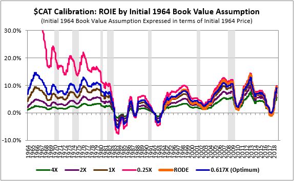
As you can see in the chart, all of the calculated ROIEs converge on the RODE over time, regardless of the initial equity assumptions used to calculate them. That's because the effects of errors in the initial equity assumptions tend to shrink as time passes. As the company grows in real terms, its distant prior equity becomes a smaller and smaller contributor to its subsequent equity, reducing the impact of any initial inaccuracies.
Some of the calculated ROIEs, however, do a better job of converging on the RODE than others. The ROIE calculated using an initial 0.25X estimate, shown in pink, does an especially poor job in that respect--it overshoots the RODE across the entire range of the chart, generating absurdly high ROIE numbers in the early periods. We can therefore throw it out as an incorrect estimate. The 4X estimate, shown in green, does the opposite. It significantly undershoots the RODE, producing deeply depressed ROIE numbers in the early periods of the chart. We can throw it out by the same logic.
What we're searching for, in the end, is the initial equity assumption that leads to the smallest possible square difference between the calculated ROIE and the RODE. In the case of $CAT, that estimate ends up being 0.617X. In other words, if we assume that $CAT's true, inflation-adjusted equity value in 1964 was 0.617 times its inflation-adjusted price on that date, and we implement the integrated equity methodology based on that assumption, the subsequent ROIEs that we calculate will exhibit the closest possible match with the subsequent long-term RODEs.
We've therefore found a solution to the initial equity problem. We can use the RODE as a calibration tool to solve for the critical missing link in the integrated equity calculation--i.e., the initial inflation-adjusted equity value. In doing this, we're effectively backfitting the initial equity assignment to produce a result that's consistent with reliable return on equity data obtained through a different method, the RODE method.
Some readers might object that this approach involves cheating because it uses future data to infer past data. But using future data to infer past data is only cheating if the inferred past data is then used to predict the future data all over again, in a circle. We're not making any predictions here. All we're doing is studying the past. We're extrapolating an observed trend backwards from the future into the past, to figure out where things were in the past. That's a perfectly valid approach to use in acquiring knowledge.
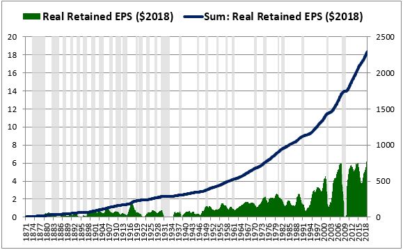
Now, let's see what happens when we use this same approach to calculate an ROIE for the S&P 500. We start by calculating the EPS that the S&P 500 retained on each date in its history (green). We then inflation-adjust that EPS to 2018 prices and calculate its running sum across the period:
We then calculate the index's RODE for periods ranging from 1871 through every future date:
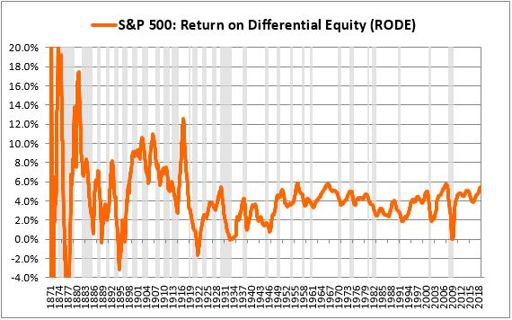
As expected, the initial numbers end up being erratic, so we cut them off, limiting the analysis to periods that end on distant future dates--in this case, dates after 1950:
We then test out different numbers for the initial January 1871 equity value, using those numbers to compute different return on integrated equity (ROIE) series. We pick the value associated with the ROIE series that most closely matches the RODE:
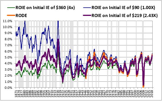
The S&P's actual inflation-adjusted price in January 1871 was $90. If we use that number as the initial equity value for the index, we get the ROIE series shown in blue. That series is unreasonably high in the early periods of the chart and overshoots the RODE in the later periods. We can therefore rule out $90 as an initial equity estimate.
If we try out a much larger number--say, $360, 4 times the index's January 1871 price--we get the ROIE series shown in green. It's unreasonably low in the early periods of the chart and undershoots the RODE in the later periods. So we can rule out $360 by the same logic.
We continue to computationally evaluate different initial equity values in this way, eventually converging on a maximally accurate initial value. In this case, that value ends up being $219--2.43 times the initial 1871 price. If we use $219 as the index's initial 1871 equity value, we get the ROIE series shown in purple. It exhibits the closest possible match with the RODE, minimizing the square difference between the lines. Conveniently, it also produces reasonable, balanced, symmetric numbers in the early period of the chart, numbers that are very likely to be correct, at least to a first approximation.
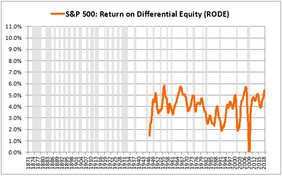
At the end of the process, we end up with the clean, orderly, mean-reverting chart shown below:
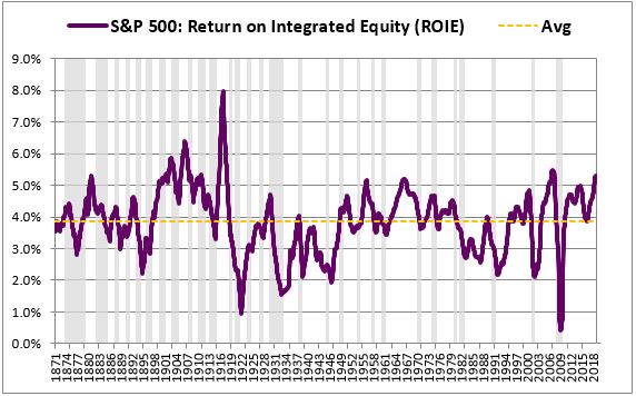
When applied to a large, well-diversified index with a long history such as the S&P 500, the integrated equity methodology tends to be very accurate, especially in later years of the analysis, after the index has had time to accumulate large amounts of retained EPS.
Whitepaper Links