Alpha within Factors
By Chris Meredith, Jesse Livermore+, Patrick O’Shaughnessy
November 2018
In Factors from Scratch, we showed that value investing works through a re-rating process. The process begins when the market develops an expectation that the earnings of certain companies will decline or grow at depressed rates into the future.1 The market then prices those companies at a discount relative to their current earnings, turning them into "value stocks." Over the short-term, the market usually ends up being right in its expectations: value stocks usually do go on to experience declines or slowdowns in their earnings, particularly in comparison with the rest of the market. But over the long-term, they usually recover and return to normal growth. When the market prices value stocks, it tends to underestimate the likelihood and extent of their eventual recoveries. Consequently, it tends to underprice them relative to the actual stream of future earnings that they go on to generate. As the future takes shape, the market adjusts to correct this mistake, re-rating the stocks higher and delivering excess returns to those who buy at the beginning of the process.
To be clear, this narrative describes the average outcome of value stocks as a group. Actual individual outcomes inside that group tend to be well-dispersed, with stocks in the group frequently taking paths that deviate from the average. Some value stocks, for example, experience strong earnings growth from the outset, as if they were growth stocks. Unsurprisingly, these stocks, which were initially priced for future earnings weakness, go on to experience large upward re-ratings, generating strong gains for investors. Other value stocks, in contrast, experience earnings declines that exceed even the market's worst expectations, without any subsequent recoveries. Predictably, these stocks get re-rated in the opposite direction, producing losses for investors.
The wide dispersion of outcomes observed in value stocks represents a significant opportunity for investors. We're going to explore that opportunity in this piece. The piece will contain two sections:
(1) In the first section, we're going to analyze and quantify the impact that future earnings outcomes have on the returns of value stocks.
(2) In the second section, we're going to introduce and evaluate a simple quantitative investment strategy that improves on the returns of a conventional value strategy by tilting its exposure in the direction of value stocks with the highest future earnings growth.
The earnings-related theme that we're going to explore in the piece is an instance of a larger theme that we've been focused on as a firm--the pursuit of "Alpha within Factors." To achieve differentiated returns, quantitative investors need to do more than just expose their portfolios to popular factors such as value and momentum. They need to implement strategies that can separate good outcomes from bad outcomes within those factors. We believe that the successful development and utilization of such strategies represents the future of quantitative investing.
Section 1: Growth in Value
Real and Fake Value: The Cases of $AAPL and $IBM
For a real-world illustration of the different fundamental paths that value stocks can take after they are purchased, consider the examples of two well-known technology companies: Apple ($AAPL) and IBM ($IBM). In June of 2014, both of these companies had trailing-twelve-month (ttm) price-to-earnings (P/E) ratios in the cheapest quintile of the large cap universe, with $AAPL trading at a ttm P/E of 14.9 and $IBM trading at a ttm P/E of 11.2. The reason the companies traded at low multiples of their current earnings is that market participants were concerned that the earnings might not be sustained (if distributed) and might not grow at normal market rates (if reinvested) over time.
The table below quantifies the performance of the two companies from June 30th, 2014 through October 30th, 2018, showing the month-end total return index ("TR"), price, P/E, ttm earnings per share ("EPS"), and ttm net income in billions of dollars ("NI"):
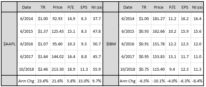
As you can see in the left portion of the table, $AAPL went on to grow its earnings at an impressive 15.0% annual rate over the period.2 This growth wasn't expected in 2014, which is why an upward adjustment in the company's price and valuation occurred. In the end, the ensuing adjustment generated a total return of 23.6% per year for continuous holders of the stock. An annually rebalanced value strategy would have invested in the stock on each rebalancing date from 2014 through 2018, earning the 23.6% return in its entirety and experiencing only one year of negative performance.
Unfortunately, the future didn't play out as well for $IBM investors. Instead of growing over the period, $IBM's earnings declined, shrinking at a rate of -6.3% per year.3 When evaluating the severity of this decline, it's important to remember that the company reinvested the majority of its earnings during the period into capital expenditures and share buybacks. The -6.3% number includes the growth benefits of that reinvestment, suggesting that the performance of the core business was even worse. Given this outcome, there wasn't any reason for the stock to be re-rated higher. To the contrary, it needed to be re-rated lower, which is what happened. Despite four years of earnings reinvestment, the price fell from $181.27 to $115.40, generating a loss of -6.5% per year for investors, -17.2% relative to the market.
The examples of $AAPL and $IBM illustrate an important and obvious truth that often gets missed in conversations about value. Value works when it's real--i.e., when stocks priced cheaply relative to their current earnings sustain and grow those earnings over the long-term. Value fails when it's fake--i.e., when stocks priced cheaply relative to their current earnings suffer declines in those earnings that never get recovered. In hindsight, we can see that the value in 2014 $AAPL was real while the value in 2014 $IBM was fake. The results for investors played out accordingly.
The Impact of Future Growth
The chart below offers a dramatic illustration of the difference between real and fake value. To construct it, we build an equally-weighted, annually-rebalanced value factor portfolio consisting of the cheapest quintile of large cap stocks on the P/E ratio. On each June rebalancing date, we look out one year into the future and divide the portfolio into two bins based on EPS growth over the upcoming holding period, with the first bin containing stocks that rank in the top half on future EPS growth and the second bin containing stocks that rank in the bottom half. We repeat this exercise in each June month from 1965 through 2017, tracking the cumulative total returns of the two bins:
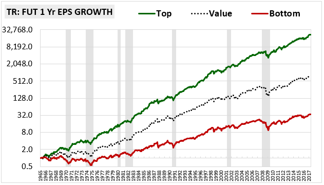
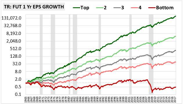
As you can see in the chart, the top-half growth bin, shown in green, dramatically outperforms the bottom-half growth bin, shown in red. As we increase the number of bins, the return differentiation increases. In the chart below, we increase the number of bins from 2 (halves) to 5 (fifths):
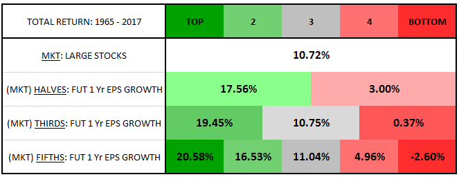
The following table quantifies the performance, showing annualized total returns for the market, the value factor and the value factor separated into halves, thirds and fifths based on future one-year EPS growth:
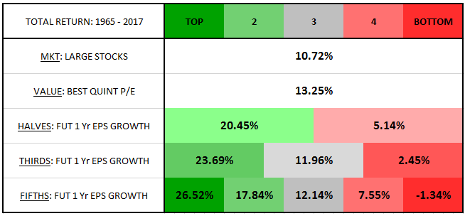
As the table makes clear, future earnings outcomes have an enormous impact on the return performance of the value factor. The simple act of dividing the factor into two halves based on future growth is enough to split the return into a massive 20.45% per year on one end and an unimpressive 5.14% on the other. As the number of bins is increased, the spread grows larger. On fifths, for example, the top-ranked bin generates an eye-popping return of 26.52% per year while the bottom-ranked bin generates a loss of -1.34% per year.
Investors in the real world don't have the ability to look into the future and distinguish stocks based on future growth outcomes. The exercise that we're engaging in here may therefore seem like pointless cheating. It's definitely cheating, but it's not pointless. It provides a powerful demonstration of the importance of future earnings outcomes in the generation of the value premium. It clarifies the basic challenge that value investors face: that of finding cheap stocks whose earnings are going to grow.
For interested readers, we've written an appendix in which we separate the returns of each of the above bins into contributions from multiple expansion and earnings growth. We use the results to gain additional insights into the value factor's inner workings.
The Market as a Control Case
Information about future earnings growth is important not just to value investing, but to all investing. A stock, after all, is nothing more than a stream of future earnings, a portion of which gets paid out to the owners and a portion of which gets reinvested into the future growth of the stream. If we know the amount of the future stream and we know the current price, then, fundamentally, we know everything that there is to know about the stock.4 For this reason, we should expect to see strong return differentiation emerge when any investment strategy is separated out based on future earnings outcomes--not just the value factor, but all investment strategies. If we want to draw particular conclusions about the return differentiation observed within the value factor, we need to compare it to a control case.
A great control case to use is the market itself. We show results for that control case in the table below, conducting the same forward-looking exercise on the equal-weighted large cap market that we conducted on the value factor. In each June month, we look out one year into the future and separate the stocks in the market into different bins based on their future one-year EPS growth numbers:
As expected, we see a similar pattern of differentiation, with the top growth bins generating significantly stronger returns than the bottom growth bins. However, when we compare these results to our earlier results for the value factor, we notice an interesting difference: the value factor receives a greater relative contribution from its top growth bins than the market receives. The table below makes this difference more clear. It shows the annualized geometric excess return5 of each value factor growth bin over the corresponding market growth bin:
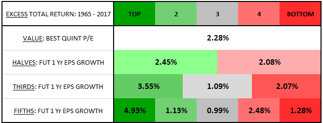
As you can see, the excess return of the value factor over the market is noticeably larger for the top growth bins than for the other growth bins. On fifths, for example, the top value factor growth bin earns an extra 4.93% per year over the top market growth bin, whereas the other value factor growth bins only earn between 0.99% and 2.48% over the corresponding market growth bins.
Another noticeable difference is that the spreads between the returns of the top growth bins and the returns of the bottom growth bins are more pronounced inside the value factor than inside the market. The table below highlights this difference by showing the annualized geometric top-over-bottom value factor return spreads alongside the same spreads for the market on six different future one-year growth partitionings: halves, thirds, fifths, tenths, twentieths, and fortieths:
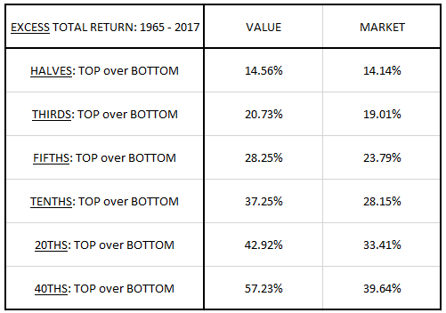
As you can see, the spreads are consistently larger in the value factor than in the market, and they increase more in the value factor than in the market as the partitionings are increased. The implication is that information about future growth outcomes is more powerful and more valuable when investing in cheap stocks than when investing in the market more generally.
Growth Bin Contributions Across History
Because the different growth bins of the value factor are equally-weighted partitions of an equally-weighted factor, the factor itself can be represented as a collective "sum" of all of the bins. We can use this fact to decompose the value factor's annual returns into separate contributions from each bin, comparing the current contributions to the historical contributions and drawing conclusions about the drivers of fluctuations in the factor's performance over time.
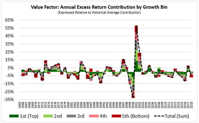
In the chart below, we show the excess return contribution of each growth bin of the value factor over the return of the broad market (just the simple return of the broad market itself, with no further differentiation based on market growth bins) in each year from 1966 through 2018. The return contribution associated with each year is the contribution from June of the prior year to June of that year. The sum of the different contributions, represented as the dotted black line, is just the excess return of the overall value factor itself:
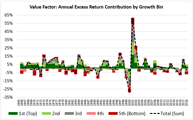
Unsurprisingly, the top growth bins (green, light green) tend to make strong positive contributions to the factor's returns, while the bottom growth bins (red, pink) tend to make negative contributions. The contribution from the middle growth bin (gray) leans positive, but also tends to oscillate from positive to negative in a way that mirrors the factor's overall performance (which is obviously impacted by the oscillations). On the whole, the factor tends to outperform because the positive contributions from the top and middle growth bins tend to outweigh the negative contributions from the bottom growth bins.
In the chart below, we show the excess return contribution of each growth bin relative to its historical average contribution. We're looking to see how the contributions have fluctuated over time relative to their historical norms:
Looking specifically at the most recent period of the chart, we notice an interesting change. The contributions from the top growth bins have frequently been negative during the period, suggesting that those bins have failed to contribute as much to the value factor's returns as they did in the past.
To make the change easier to see, the chart below averages the contributions of each growth bin over trailing five-year periods. The recent area of weakness is circled in blue:
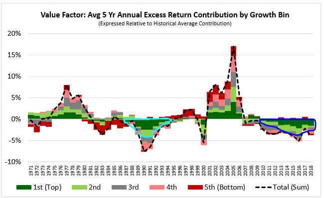
As you can see, the recent contribution from the top growth bin has been strongly negative relative to its historical average--indeed, more negative than the contributions from the bottom bins.
When the value factor underperforms, our inclination is to blame the underperformance on the trashier parts of the factor, i.e., the "value traps" that sit in its lower growth bins. But those bins aren't always to blame. As we see in the most recent period, the underperformance can just as easily emerge out of weakness in the factor's higher growth bins, which sometimes fail to add to returns in a way that is consistent with their histories. If the positive contributions from the higher growth bins drop off substantially, then there won't be anything to offset the natural weakness found in the lower growth bins, and the factor itself will tend to underperform.
We should note, in passing, that the recent weakness in the value factor's higher growth bins is not a new phenomenon. As you can see in the area circled in aqua, weakness from those bins was also an important contributor to the extended period of underperformance that the factor experienced in the late 1980s.
Section 2: Capturing the Returns
The challenge in value investing is to identify real value--i.e., stocks priced cheaply relative to current earnings that will sustain and grow those earnings over time. The question, of course, is whether we can meet that challenge using presently-available information alone. Up to now in the piece, we've been meeting it by cheating, by allowing ourselves to go into the future and identify the targeted stocks in hindsight. In the real world, that isn't an option.
Is it possible to reliably identify the top-growing stocks in the value factor using presently-available information? The answer is surely no, especially if presently-available information is limited to price and financial statement data. The forces that determine future earnings outcomes in businesses arise out of complex, idiosyncratic chains of causality that are not fully captured in that data.
But the point is, to do well as value investors, we don't need to reliably identify the top-growing stocks in the value space. All we need to do is tilt our portfolios in their direction, however slightly. As we saw earlier, the top growth bin of the value factor generates a historical return of more than 26% per year, 16% above the market. If we could manage to capture even a small fraction of that return, we would be doing very well.
Our challenge, then, is to find realistic ways to tilt a portfolio of value stocks in the direction of stronger future growth outcomes. In this section, we're going to introduce and analyze a simple three-step quantitative strategy that seeks to achieve that goal. OSAM doesn't actually use the simplified strategy that we're going to share, but it uses strategies that are based on similar concepts.
Step 1: Improving the Measurement of Value
The first step in the strategy is to improve the measurement of value. Valuation metrics that compare the price of a stock to some fundamental (e.g., earnings, sales, book value, etc.) face the problem of selection bias. By definition, they are biased to select companies with exaggerated or overstated expressions of that fundamental. The market knows that the fundamental is overstated, and therefore correctly prices the stock cheaply relative to it. But the valuation metric doesn't know this, and therefore wrongly concludes that the stock actually is cheap.
For a highly-relevant recent example of the problem of selection bias, consider the case of Berkshire Hathaway ($BRK-B). If you go online and check the P/E ratio of $BRK-B, you will see that it's unusually low--as of October 2018, the stock is trading at around $205 against trailing earnings of around $19, a multiple of roughly 11 times. A value strategy defined on the P/E ratio will therefore identify $BRK-B as a value stock and bring it into the portfolio. But when we examine $BRK-B's income statement, we find that the $19 number is illusory, the result of a large one-time tax gain taken in the fourth quarter of 2017.
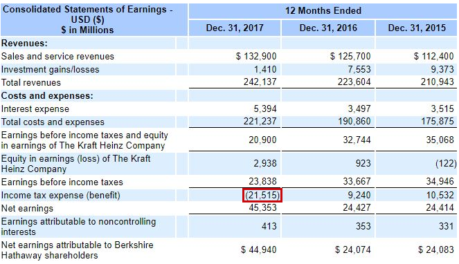
The market knows that $BRK-B's recurring future earnings will be significantly less than $19, which is why it is pricing the stock cheaply relative to that number. But the value factor as we've defined it can't tell the difference. It stupidly invests in $BRK-B, thinking that it's getting a bargain.
The Trump tax cuts passed at the end of 2017 have made tax-related accounting distortions such as the one seen in $BRK-B unusually common over the last year. These distortions have caused some investors to wrongly conclude that the value factor is generationally cheap relative to the market. But the apparent cheapness is illusory, a non-recurring consequence of a one-time change in government policy.
The problem with selection bias in the value factor is not that it necessarily causes losses, but rather that it weakens the signal that the factor is trying to capture. Berkshire Hathaway is an excellent company and could very well turn out to be a fantastic investment at its current price. But it's not the value stock that it appears to be. Absent specific information about it, we'd have to say that it's just market beta. When it gets inadvertently introduced into a value portfolio, it ends up diluting the exposure that the portfolio is trying to achieve.
A secondary problem with selection bias in the value factor is that it sets the factor up for illusory future earnings declines. Several months from now, when $BRK-B's one-time tax benefit has dropped out of the trailing-twelve-month period, the company will likely be earning something in the area of $10 per year, which means that it will officially experience a 50% decline in its earnings from current levels. Of course, this decline isn't going to be real, and therefore isn't going to hurt anyone, but it will distort the value factor's EPS profile, creating the appearance of a large drop that didn't actually happen.
It goes without saying that quantitative investors should try to represent the fundamentals that they are using in their valuation metrics in the most accurate way possible. In the case of $BRK-B, this would mean ensuring that one-time tax gains are taken out of the earnings measure. But the process of trying to exclude overstatements and exaggerations can quickly turn into a game of "whack-a-mole", where an attempt to eliminate a potential distortion in one area of the market ends up creating a different distortion in another. The problem is especially hard to solve when working with several thousands of companies across several decades of historical data.
A more practical solution, then, is to build a composite measure of valuation that averages the inputs of different valuation metrics together. Then, if a company wrongly appears cheap on one particular metric, as $BRK-B did, it won't get drawn into the portfolio, because it will have registered as not being cheap on the others.
At OSAM, we measure valuation using a composite index that takes inputs from the P/E ratio, the enterprise-value-to-ebitda ratio, the enterprise-value-to-free-cash-flow ratio and the price-to-sales ratio.6 In testing, we've found that this approach generates excess returns that are smoother and more consistent than the metrics in isolation.
From here forward, when we refer to the "value factor", we will no longer be referring to the cheapest quintile of large cap stocks on the P/E ratio. Instead, we will be referring to the cheapest quintile of large cap stocks on our composite index, as defined above. Note that this change will lead to changes in the value factor's performance in certain periods relative to the results shown in prior charts and tables.
Step 2: Removing Value Traps
The second step in the process is to remove companies that are statistically likely to exhibit future fundamental weakness--companies that we will pejoratively refer to as "value traps." To identify value traps, we score companies in the investment universe on four simplified indices:
(1) Momentum: a measure of trailing total return; higher is better.
(2) Growth: a measure of trailing change in earnings; higher is better.
(3) Earnings Quality: a measure of accruals; lower is better.
(4) Financial Strength: a measure of leverage; lower is better.
As a rule, we remove any company that scores in the bottom 10th percentile of the market on any of these indices. We use a low percentile as the cutoff point because we want to maximize the number of stocks remaining in the factor, so as to maximize the statistical reliability of the result. The strategy is able to substantially improve the performance despite a low cutoff point because the indices exhibit their greatest predictive power at the bottom end of the spectrum--that is, they predict bad stocks better than they predict good stocks, and the predictions get better as the rankings get lower.
In the table below, we highlight the performance differences between value stocks, value traps and the large cap market by calculating a series of arithmetic averages for each category. More specifically, we calculate the arithmetic average excess total return over the next year of every value stock, every value trap, and every large cap stock that existed between December 1962 and May 2017.7 We also show the allocation of value traps to each future EPS growth bin of the value factor--i.e., the percentage of value trap stocks that were also stocks in those value factor growth bins:
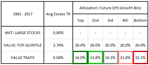
Calculating arithmetic averages is a slightly inaccurate way of depicting returns, but in this case, it's sufficient to capture the relevant performance differences. As a group, value stocks generate a 2.74% average excess return over the market, while value stocks that meet value trap criteria generate an average excess return of only 0.04%--essentially no excess return at all. The losses associated with being a value trap, then, are large enough to erase the value premium altogether.
Looking at the area boxed in red, we see that the poor performance of value traps is associated with a substantial increase in allocation to the bottom growth bin of the value factor. A full 32.1% of value traps are stocks that come from that bin, in comparison with 20% of value stocks more generally. The increased allocation to the bottom growth bin is mirrored by a notable decrease in allocation to the median and top growth bins, boxed in gray, light green, and dark green, respectively.
In the table below, we show the future one-year EPS growth profiles of the different categories of stocks. The numbers are calculated over one year periods that begin in each month and that extend out to the same month one year later. We express the growth profiles in the form of average percentile marks, ranging from the 10th percentile to the 90th percentile.8 In the right hand column, we show the average of all of the percentile marks:
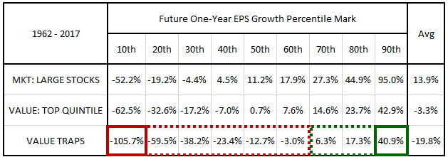
As you can see, value stocks that meet value trap criteria exhibit a future growth profile that is significantly more negative than the profiles of the market and the larger value universe. They go negative at the 60th percentile rather than the 30th and 40th percentiles, respectively, and they suffer extreme losses on the lower tail end of the distribution. Their percentile marks average to -19.8%, significantly lower than the average 13.9% and -3.3% observed in the market and the larger value universe, respectively.
The evidence confirms that value traps, which we've identified using simple, currently-observable data points, expose us to more of the bad parts of the value factor and less of the good parts--a tendency that explains their weak returns. We have no reason to want them in our portfolios, so we take them out.
The table below shows the arithmetic average excess total return and future growth bin allocation of the value factor with value traps removed ("Value ex Traps"):
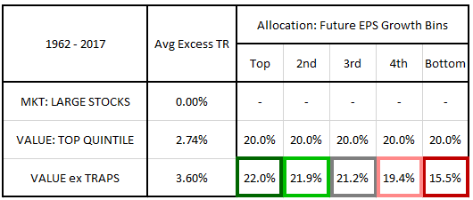
The average excess return increases from 2.74% to 3.60%, a gain of 0.86%. As expected, the improvement is associated with a significant reduction in the value factor's allocation to the bottom growth bin, which falls from 20.0% to 15.5%.
In the table below, we show the future one-year EPS growth profile of the value factor with value traps removed:
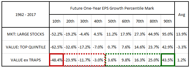
The lower percentile marks increase significantly, suggesting that the removal is chopping off a substantial portion of the negative left tail of the value factor's EPS growth distribution. Surprisingly, with value traps removed, the 10th percentile of EPS growth in the value factor ends up being higher than the market's 10th percentile, coming in at -48.4% versus the market's -52.2%. This is a noteworthy improvement considering that value stocks tend to have future growth profiles that are substantially more negative than the growth profiles of the market.
Step 3: Selecting the Best of What Remains
The third step in the process is to select the highest ranking value stocks out of what remains once the value traps have been removed. To do this, we average the index scores of each company together to form a composite score. We then select the top half of the remaining stocks based on that composite score. We refer to those stocks as "value leaders" and make equal-weighted investments in them to form the final portfolio.
The table below shows the average excess return and future growth bin allocations of value leaders as a group:
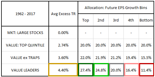
Value leaders generate an average excess return of 4.40% per year, 1.66% higher than the value factor's 2.74% return. The increase in return coincides with a substantial increase in exposure to the value factor's top growth bin (20.0% to 27.4%) and a substantial decrease in exposure to the value factor's bottom growth bin (20.0% to 11.4%).
In the table below, we show the future one-year EPS growth profile of value leaders:
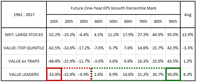
As you can see, the percentile marks for the value leaders strategy are higher than the percentile marks for the value factor at every percentile. The overall average of the marks is +8.3%, a significant improvement over the value factor's -3.3%.
Summarizing the Results
In the table below, we show the future value factor growth bin allocations of all of the strategies that we've analyzed up to this point. Recall that these allocations simply denote the share of stocks in each strategy that fall into the different future EPS growth bins of the value factor. For reference, we've included the allocations of the top and bottom growth bins themselves:
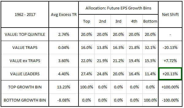
In the far-right column of the table, we show the net shift of each strategy towards a full allocation to the top value factor growth bin.9 The scale is defined such that a +100.00% net shift signifies that the strategy has moved from an equal allocation to a 100% top growth bin allocation. A -100.00% net shift signifies the opposite--a shift from an equal allocation to a 100% bottom growth bin allocation.
As you can see in the cell boxed in green, the value leaders strategy exhibits a net shift of +20.13%--an impressive number, considering that it's using only presently-available information. The strategy may not be able to perfectly predict the top-growing value stocks in advance, but it's able to strongly tilt the allocation in their direction, which was the goal that we specified at the outset.
In the table below, we present statistical results for the strategies:
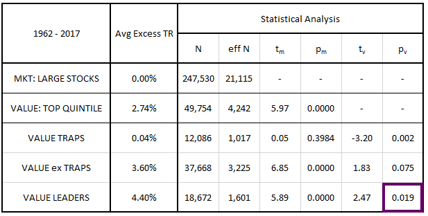
Value traps represent roughly 25% of the value universe, with non-trap value stocks representing the remaining 75%. Value leaders represent half of the non-trap value stocks, or roughly 38% of the overall value universe.
The sample sizes ("N") in the analysis are extremely large, but they contain overlapping monthly results--for example, they include $AAPL's returns from January of 2008 to January of 2009, February of 2008 to February of 2009, March of 2008 to March of 2009, and so on. Because these results overlap with each other, they do not represent fully independent samples of the space. To be maximally conservative, we've therefore calculated the t-stats and p-values using effective sample sizes ("eff N"), defined as the number of non-overlapping June-to-June samples (roughly one-twelfth of the larger sample sizes).
The columns labeled "tm" and "pm" show the t-stats and p-values of each strategy when tested against the market. The results are not particularly informative, however, because the strategies were built from the value universe and therefore already contain the excess returns of the value factor within them. The strategies therefore need to be tested against the value factor itself. We show the results of tests of the strategies against the value factor in columns "tv" and "pv." As you can see, the excess return of the value leaders strategy over the value factor is statistically significant to the 0.05 level.
In the table below, we show the future one-year EPS growth profiles of all of the strategies. The numbers in the columns are averages of the EPS growth values that demarcated the specified percentiles in the strategies across history, from the 10th percentile to the 90th percentile:
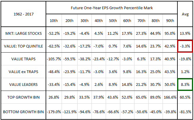
Relative to the value factor, the value ex trap and value leaders strategies exhibit increased future EPS growth profiles at all percentiles, achieving the largest improvements at the lower end of the distribution.10
Different Periods of Market History
In the table below, we show the excess returns of the different strategies across different periods of market history:
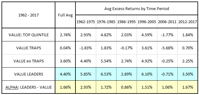
We define the "alpha" of the value leaders strategy as the difference between its excess return and the excess return of the value factor. As you can see, the value leaders strategy generated positive alpha in every period analyzed. It also beat the overall market in every period except 2006 to 2011, which was the period that overlapped with the financial crisis.
The table below shows the allocation of the value leaders strategy of to the different growth bins of the value factor in each period:
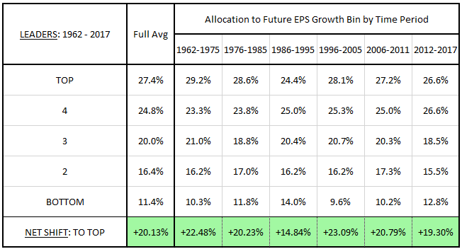
We stated at the outset that our goal was to use presently-available information to shift the allocations of the value factor towards higher future growth bins. As you can see in the table, the value leaders strategy consistently achieves that goal. The net shift is roughly 20% or higher in every period of the table. The one exception is the period from 1986 to 1995 --a period that, not coincidentally, also represented the low point in the strategy's alpha.
Performance of the Value Leaders Portfolio
The excess returns shown in the tables above were determined by calculating simple arithmetic averages of the excess returns of all stocks that fell into the various strategies across history. The disadvantage to this calculational approach is that it penalizes the value leaders strategy relative to the value factor and the market. More specifically, it makes the excess returns of the value leaders strategy over those strategies appear smaller than they actually are.11 For a fully accurate assessment of the value leaders strategy's performance, we need to use a geometric approach, where we represent the strategy as an actual portfolio that compounds over time.
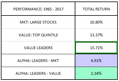
In the chart below12, we show the cumulative total returns of portfolios consisting of the equally-weighted market, the value factor and the value leaders strategy from June 1965 through March 2018. The portfolios are rebalanced annually at the end of each June month:
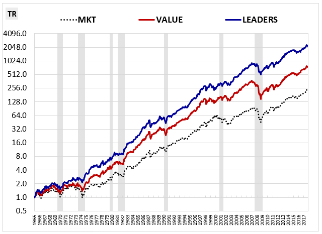
All told, the value leaders strategy generates a compound annual total return of 15.71%, 4.91% above the equally-weighted large cap universe and 2.34% above the value factor:
Using the methods introduced in Factors from Scratch, we can decompose the total returns of the strategy into contributions13 from holding period multiple expansion and holding period EPS growth. The results are presented in the table below:
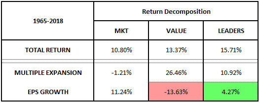
The improvement in returns is associated with an increase in holding period EPS growth from negative 13.63% to positive 4.27%. With this increase, the strategy is achieving the goal that we specified at the outset. It's improving the returns of the value factor by tilting the factor's exposure in the direction of value stocks with stronger future earnings growth.
The outperformance of the value leaders strategy is notable for three reasons:
First, it requires only a modest amount of intervention. The percentage of original value stocks retained in the final strategy--38%--is relatively large. Moreover, the strategy is rebalanced annually, rather than quarterly or monthly. These characteristics suggest that the strategy is able to accomplish more with less.
Second, it's occurring entirely in the large cap space, a space in which factor signals are comparatively weak and, according to some, non-existent.
Third, it's associated with a significant shift in allocation towards the value factor's top growth bins, a shift that we know is efficacious, given the extreme levels of outperformance produced by stocks in those bins.
Conclusion—Where We Go From Here
As investors, our goal is to understand and capitalize on every advantage available to us in markets. The discovery of primary factors--e.g., value and momentum--represented an important step toward that goal.
The next step is alpha within factors.
In this piece, we showed that it's possible to generate alpha within the value factor by shifting its allocation in the direction of stocks with better future earnings outcomes. We used additional factors that are correlated with those outcomes--specifically: momentum, trailing growth, accruals and leverage--to filter out value traps and identify the strongest companies out of what remains. The reality, of course, is that these additional factors are well-known and widely implemented in markets. In practice, we therefore use methods that are more focused and refined. We also take advantage of the benefits of concentration and size: factor investing is more powerful when applied in a concentrated manner and when used outside of the large cap space.
The advantage to focusing on future earnings outcomes in the context of value investing is that it moves the process beyond the trivial phase, into an area that actually requires expertise. It's easy to find stocks with low P/E ratios, but it's hard to determine whether those stocks will sustain and grow their earnings into the future. For skilled investors, that's a good thing--harder challenges mean less competition and a greater opportunity to outperform.
As quantitative investors, our basic approach to finding alpha is the scientific method. We use observation and analysis to identify hypotheses that are likely to be true. We then rigorously test those hypotheses in data, always treating the data as the absolute and final arbiter. But there's another approach that can be used to that end--the approach of differentiated modeling, commonly referred to as "machine learning." In machine learning, we let a computer algorithm come up with a hypothesis by allowing it to train on a subset of the data. We then test and validate what it comes up with on other subsets of the data that it has yet to see. Our next paper will examine simple but powerful ways in which machine learning can be used to identify alpha within factors.
In investing research, knowing what to search for is half the battle. The quantitative industry has traditionally searched for companies with strong future returns. But as we've shown in this piece, sometimes a better way to find those companies is to search for strength in a different, more predictable variable: future fundamental growth. We believe that identifying variables that lead to differentiated returns within factors is a great way to improve factor investing. We look forward to sharing future findings with you as we continue to explore this promising area of research.
Appendix
Footnotes
1 We focus on earnings in this piece, but other economically-relevant fundamentals--e.g., EBITDA, free cash flow, sales, book equity, etc.--can be used in its place.
2 Approximately 5.3% of $AAPL's 15.0% annual EPS growth was due to the share-count-shrinking effect of net share buybacks. The other 9.7% was organic.
3 The 10/2018 numbers shown in the table exclude a large tax charge that $IBM took in the 4Q of 2017.
4 This point assumes that the earnings have been accurately reported and that they are going to be appropriately stewarded by whoever controls their allocation.
5 To calculate the annualized geometric excess return, we take the cumulative, non-annualized total return of the specified growth bin of the value factor and divide it by the cumulative, non-annualized total return of the associated growth bin of the market. We then annualize the resulting ratio.
6 We exclude the popular price-to-book ratio because we believe that it does more harm than good. For an extensive analysis of its shortcomings, see this recent piece by our colleague Travis Fairchild.
7 The excess return over the next year of a given stock in a given month is defined relative to the return over the next year of the rest of the market in that month.
8 We calculate the average percentile marks by computing the actual percentile marks in each month and then averaging all the months together across history.
9 We define the net shift as the change in the allocation to the top bin plus half the change in the allocation to the 2nd bin minus half the change in allocation to the 4th bin minus the change in allocation to the bottom bin.
10 The average number shown in the right hand column is not the actual average future EPS growth, but rather the average of the 10th through the 90th percentile marks. If computed on all stocks, the actual average number would be lower because EPS growth at the far left end of the distribution is disproportionately negative.
11 Arithmetic averaging numerically boosts returns relative to geometric averaging. The boosts tend to be greater when the variance of the series is greater. Because the returns of the value factor and the returns of the market exhibit greater variance than the returns of the value leader strategy, they get larger boosts from the arithmetic averaging. Consequently, the excess return of the value leaders strategy over those benchmarks ends up appearing smaller.
12 We exclude the 1962 through 1965 period because the number of stocks in that period is too small to support a robust analysis.
13 Using the terminology of the piece, the return from holding period multiple expansion is just the rebalancing growth and the return from holding period EPS growth is just the holding growth. These returns do not exactly add up to the total return because there is a small return contribution from unrebalanced (end-to-end) change in valuation. To keep things simple, we've left that contribution out of the table.
GENERAL LEGAL DISCLOSURES & HYPOTHETICAL AND/OR BACKTESTED RESULTS DISCLAIMER
The material contained herein is intended as a general market commentary. Opinions expressed herein are solely those of O’Shaughnessy Asset Management, LLC and may differ from those of your broker or investment firm.
Please remember that past performance may not be indicative of future results. Different types of investments involve varying degrees of risk, and there can be no assurance that the future performance of any specific investment, investment strategy, or product (including the investments and/or investment strategies recommended or undertaken by O’Shaughnessy Asset Management, LLC), or any non-investment related content, made reference to directly or indirectly in this piece will be profitable, equal any corresponding indicated historical performance level(s), be suitable for your portfolio or individual situation, or prove successful. Due to various factors, including changing market conditions and/or applicable laws, the content may no longer be reflective of current opinions or positions. Moreover, you should not assume that any discussion or information contained in this piece serves as the receipt of, or as a substitute for, personalized investment advice from O’Shaughnessy Asset Management, LLC. Any individual account performance information reflects the reinvestment of dividends (to the extent applicable), and is net of applicable transaction fees, O’Shaughnessy Asset Management, LLC’s investment management fee (if debited directly from the account), and any other related account expenses. Account information has been compiled solely by O’Shaughnessy Asset Management, LLC, has not been independently verified, and does not reflect the impact of taxes on non-qualified accounts. In preparing this report, O’Shaughnessy Asset Management, LLC has relied upon information provided by the account custodian. Please defer to formal tax documents received from the account custodian for cost basis and tax reporting purposes. Please remember to contact O’Shaughnessy Asset Management, LLC, in writing, if there are any changes in your personal/financial situation or investment objectives for the purpose of reviewing/evaluating/revising our previous recommendations and/or services, or if you want to impose, add, or modify any reasonable restrictions to our investment advisory services. Please Note: Unless you advise, in writing, to the contrary, we will assume that there are no restrictions on our services, other than to manage the account in accordance with your designated investment objective. Please Also Note: Please compare this statement with account statements received from the account custodian. The account custodian does not verify the accuracy of the advisory fee calculation. Please advise us if you have not been receiving monthly statements from the account custodian. Historical performance results for investment indices and/or categories have been provided for general comparison purposes only, and generally do not reflect the deduction of transaction and/or custodial charges, the deduction of an investment management fee, nor the impact of taxes, the incurrence of which would have the effect of decreasing historical performance results. It should not be assumed that your account holdings correspond directly to any comparative indices. To the extent that a reader has any questions regarding the applicability of any specific issue discussed above to his/her individual situation, he/she is encouraged to consult with the professional advisor of his/her choosing. O’Shaughnessy Asset Management, LLC is neither a law firm nor a certified public accounting firm and no portion of the newsletter content should be construed as legal or accounting advice. A copy of the O’Shaughnessy Asset Management, LLC’s current written disclosure statement discussing our advisory services and fees is available upon request
The risk-free rate used in the calculation of Sortino, Sharpe, and Treynor ratios is 5%, consistently applied across time
The universe of All Stocks consists of all securities in the Chicago Research in Security Prices (CRSP) dataset or S&P Compustat Database (or other, as noted) with inflation-adjusted market capitalization greater than $200 million as of most recent year-end. The universe of Large Stocks consists of all securities in the Chicago Research in Security Prices (CRSP) dataset or S&P Compustat Database (or other, as noted) with inflation-adjusted market capitalization greater than the universe average as of most recent year-end. The stocks are equally weighted and generally rebalanced annually
Hypothetical performance results shown on the preceding pages are backtested and do not represent the performance of any account managed by OSAM, but were achieved by means of the retroactive application of each of the previously referenced models, certain aspects of which may have been designed with the benefit of hindsight
The hypothetical backtested performance does not represent the results of actual trading using client assets nor decision-making during the period and does not and is not intended to indicate the past performance or future performance of any account or investment strategy managed by OSAM. If actual accounts had been managed throughout the period, ongoing research might have resulted in changes to the strategy which might have altered returns. The performance of any account or investment strategy managed by OSAM will differ from the hypothetical backtested performance results for each factor shown herein for a number of reasons, including without limitation the following:
- Although OSAM may consider from time to time one or more of the factors noted herein in managing any account, it may not consider all or any of such factors. OSAM may (and will) from time to time consider factors in addition to those noted herein in managing any account.
- OSAM may rebalance an account more frequently or less frequently than annually and at times other than presented herein.
- OSAM may from time to time manage an account by using non-quantitative, subjective investment management methodologies in conjunction with the application of factors.
- The hypothetical backtested performance results assume full investment, whereas an account managed by OSAM may have a positive cash position upon rebalance. Had the hypothetical backtested performance results included a positive cash position, the results would have been different and generally would have been lower.
- The hypothetical backtested performance results for each factor do not reflect any transaction costs of buying and selling securities, investment management fees (including without limitation management fees and performance fees), custody and other costs, or taxes – all of which would be incurred by an investor in any account managed by OSAM. If such costs and fees were reflected, the hypothetical backtested performance results would be lower.
- The hypothetical performance does not reflect the reinvestment of dividends and distributions therefrom, interest, capital gains and withholding taxes.
- Accounts managed by OSAM are subject to additions and redemptions of assets under management, which may positively or negatively affect performance depending generally upon the timing of such events in relation to the market’s direction.
- Simulated returns may be dependent on the market and economic conditions that existed during the period. Future market or economic conditions can adversely affect the returns.