Appendix: Additional Insights into the Value Factor's Inner Workings
By Jesse Livermore+, Chris Meredith, Patrick O’Shaughnessy
November 2018
In this appendix, we're going to explore the inner workings of the value factor by analyzing the properties and behaviors of its different future growth bins. To follow the analysis, readers will need to have read our earlier piece on the topic, Factors from Scratch.
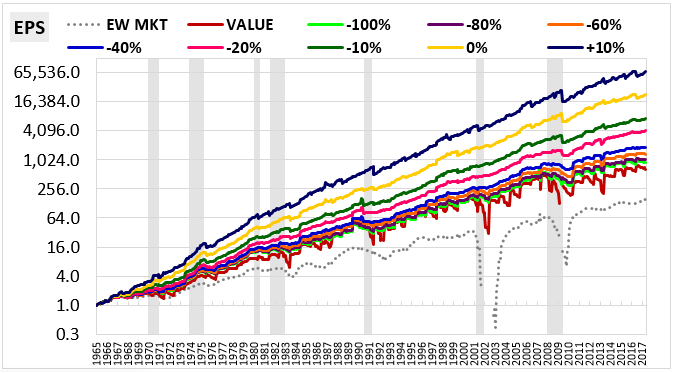
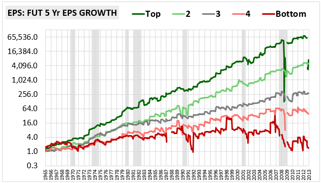
The chart below shows the EPS of the value factor and its five future one-year EPS growth bins from 1965 through 2017. The black line is the EPS of the value factor itself and the colored lines are the EPS of the different growth bins within it, ranging from the top growth bin in green to the bottom growth bin in red. The vertical gridlines delineate the June rebalancing dates:
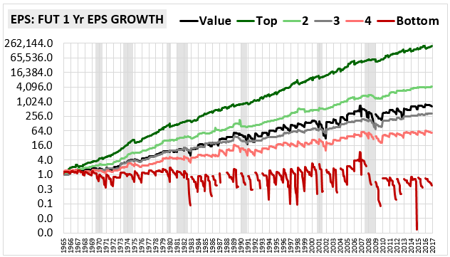
We can think of the black line as the aggregate EPS that we would end up with if we took the stocks that make up all of the other lines and threw them together into a single portfolio. If we follow the black line closely, we will notice that it declines substantially during the holding periods (the areas between the vertical gridlines). In Factors from Scratch, we calculated the average holding period decline to be -22.5% per year.
The presence of significant declines in the value factor's EPS growth profile creates the impression that value stocks are bad businesses--an impression that is partially correct. However, when interpreting the declines, we need to consider their origins. They are not being produced uniformly across the factor, but are instead emerging out of the enormous negative EPS growth contributions of the bottom growth bin, shown in blood red.
Rather than focus on the black line, we can get a better picture of the EPS profile of the "typical" value stock by examining the gray line, which represents the profile of the median future EPS growth bin. On average, the earnings of the companies in that bin are declining during the holding periods, but the declines aren't as pronounced as they are in the overall factor, which is being disproportionately weighed down by the bottom bin. Despite the small holding period declines, the EPS of the median bin is able to grow by more than the market EPS over time because it benefits from multiple expansion in the underlying companies, which shows up in the form of vertical EPS jumps that take place on the rebalancing dates.
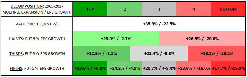
In the table below, we decompose the returns of the value factor's different growth bins into annual contributions from holding period multiple expansion and holding period EPS growth. The contribution from multiple expansion is shown on the left side of each cell and the contribution from EPS growth is shown on the right side:
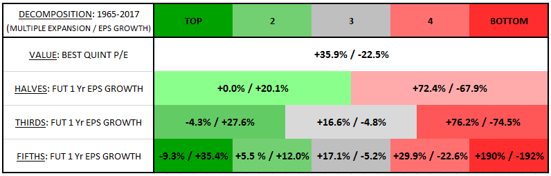
Notice that the first row has an entry of "+35.9% / -22.5%." What this means is that from 1965 through 2017, the value factor's total return separated out into an average +35.9% annual gain from multiple expansion during the holding periods and an average -22.5% annual loss from EPS declines during the holding periods. These averages are calculated over 52 holding periods in total, with each holding period beginning in June and lasting for one year.
As we move left into the higher growth bins, we find that EPS growth becomes an increasing contributor to the returns. Similarly, as we move right into the lower growth bins, we find that EPS growth becomes a diminishing contributor to the returns. This result makes sense given that we are literally defining bin membership based on EPS growth over the next year, i.e., EPS growth over the holding period of the strategy. Our partitioning therefore directly selects for the growth contributions that the table above decomposes the strategies' returns into.
What is not as clear is why the contribution from multiple expansion increases as we move into lower growth bins, and why it decreases as we move into higher growth bins. In the top third and top fifth bins, for example, the contribution from multiple expansion is negative--registering at -4.3% and -9.3%, respectively--indicating that the multiples of the stocks in those bins are actually contracting on average during the holding periods.
We see this same phenomenon--a shift from multiple expansion to multiple contraction--when we remove companies with negative future earnings growth from the value factor. The table below decomposes the value factor's returns on the assumption that all stocks with EPS growth below a specified cutoff point get removed:
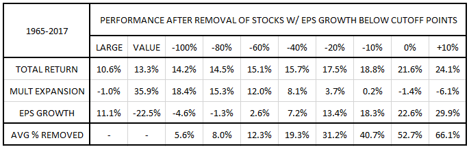
As you can see, the contribution from multiple expansion steadily falls as the as the cutoff points are shifted upwards. Eventually, when all of the negative future growers are cut out of the portfolio, the contribution from multiple expansion goes negative, turning into multiple contraction. The total return of the portfolio dramatically increases in that process, confirming the importance of future earnings growth to the value factor's performance.
The "AVG % REMOVED" row shows the average percentage of stocks removed from the value factor at each cutoff point over all years from 1965 to 2017. The actual percentage of stocks that get removed in any specific year varies significantly by year. For example, from 2008 to 2009, 36% of value stocks had earnings growth below the -100% cutoff point, whereas from 2006 to 2007 only 2% of value stocks had earnings growth below that cutoff point.
In the chart below, we show the EPS of the value factor on each of the different cutoff points:
Notice that the value factor's characteristic sawtooth EPS pattern, depicted most clearly in the red line, decays as the cutoff points are increased. At the higher cutoff points, there isn't any sawtoothing at all. The same trend can be seen in the earlier chart of the EPS of the five bins. The lower growth bins showed large amounts of sawtoothing, whereas the higher growth bins showed reduced sawtoothing (and eventually reversed sawtoothing). As we explained in Factors from Scratch, the sawtooth pattern is driven by multiple expansion. The fact that it's decaying at higher cutoff points and in higher growth bins suggests that multiple expansion is taking place to a lesser extent among the stocks in those bins.
This result poses an interesting challenge to a key thesis in Factors from Scratch. Recall that we argued that the value factor works through a re-rating process in which the future outlook for value stocks becomes less negative, causing the depressed multiples of the stocks to expand. This description is accurate for value stocks as a group, and also for the middle and lower future growth bins within it. But those bins aren't where the bulk of the value factor's excess returns come from. The bulk of the value factor's excess returns come from the top future growth bins. If the stocks in the top future growth bins aren't experiencing multiple expansion--if their multiples are, in fact, contracting--then how can the thesis be correct?
The short answer is that multiple expansion itself is not central to the thesis. What is central to the thesis is the upward re-rating process, i.e., the improvement in the future outlook that occurs during the holding periods. That improvement drives the value factor's returns. It typically occurs in conjunction with multiple expansion, but it doesn't have to occur in that way--a stock can get re-rated upward without having its multiple expand, provided that its current earnings are growing rapidly during the course of the re-rating. That's exactly what happens to the stocks in the top growth bins--sentiment towards them improves significantly, causing their prices to increase significantly, but their current earnings are growing rapidly during that same process, outpacing the price increases and causing their P/E multiples to contract (slightly).
To make this point more intuitive, we need to get clear on what a change in the P/E multiple of a stock actually conveys. That's what we're going to do in the next several paragraphs.
In theory, the "P" in the "P/E" ratio represents not only the trading price of a stock, but also the market's best estimate of the present value of its entire future stream of earnings, which we can refer to as "EALL." The "E" in the "P/E" ratio, in contrast, represents only the earnings that the stock has generated over the trailing one year period. To reiterate:
- "P" = the market price; also, the market's best estimate of the present value of "EALL."
- "EALL" = the entire future stream of earnings (expected or actual).
- "E" = the earnings generated over the trailing twelve month period.
Fundamentally, the correct "P" of a stock is determined by "EALL", not by "E." Indeed, "E" is just a backwards-looking time slice found at the beginning of the stream--it's only important to the extent that it provides an accurate projection or window into the future trajectory of the stream--i.e., an accurate representation of "EALL."
In an absolute sense, stocks become "value stocks" when the market comes to expect that their "EALL" will be lower than what is currently being projected by their "E." In the relative sense, stocks become value stocks when the difference between the market's estimation of their "EALL" and what is currently being projected by their "E" ends up being large (and negative) relative to other stocks in the market.
Given that the market sets the price "P" of the stocks based on its estimate of "EALL", if its estimate of "EALL" is low relative to what is being projected by "E", then the price "P" that it sets will also end up being low relative to what is being projected by "E." The result will be a low "P/E" ratio, which embeds a belief that current earnings ("E") either won't be sustained or won't grow at normal market rates over the long-term.
To illustrate with an example, the future earnings "EALL" of IBM ended up being significantly lower than what was projected by the company's trailing one-year earnings "E" as of June 2014. The market had a sense that the future earnings would be lower than what was projected by the trailing earnings at the time, and therefore it priced $IBM at an extremely low P/E ratio on that date. Given the earnings declines that the company went on to suffer, the market was right to price the company at a low P/E ratio. In fact, looking back, the stock's P/E ratio should have been much lower than it actually was, because the earnings declines turned out to be much worse than expected, and they were never recovered.
Now, there are two ways that a P/E multiple can expand--a good way and a bad way. Similarly, there are two ways that a P/E multiple can contract--a good way and a bad way. The table below provides a depiction of each way:
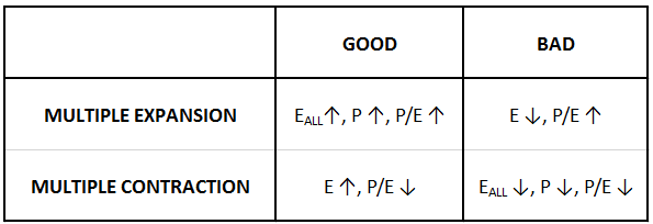
Good Multiple Expansion happens when the market's estimate of "EALL" increases, causing the price to increase. To the extent that trailing earnings stay constant in this process, the "P/E" will increase as well. This type of increase is what we're referring to when we describe value stocks as benefitting from an "upward re-rating." The market is becoming more optimistic about their future prospects--i.e., their "EALL"--and the optimism is showing up in both their "P" and their "P/E" ratio, yielding excess returns for investors.
Example: A stock trades at $20 against trailing earnings of $2--a depressed P/E multiple of 10, which expresses the market's belief that the company's trailing earnings are not reflective of its likely future earnings prospects. As more information comes in, the market shifts its view on that front, becoming more optimistic about the earnings that the company will generate in the future. The price therefore increases to $40 and the P/E multiple increases to 20. The stock ceases to be a value stock, and those who bought it when it was a value stock make money.
Bad Multiple Contraction is the reverse of Good Multiple Expansion. It happens when the market's estimate of "EALL" drops, causing the price to drop. Assuming that trailing earnings stay constant, the "P/E" will fall as well. This type of fall is what we're referring to when we talk about a "downward re-rating"--the kind of re-rating that occurred, for example, in $IBM. The market is becoming more pessimistic about a company's future prospects--i.e., its "EALL"--and the pessimism is showing up in both the "P" and the "P/E" ratio, producing losses for investors.
Example: Our earlier company is priced at $40 against trailing earnings of $2--a P/E multiple of 20. The market then becomes pessimistic about its future prospects and comes to anticipate a long-term decline in its earnings. The price therefore falls to $20 and the P/E multiple decreases to 10. The stock is now a value stock again, and those who bought it before it became a value stock lose money.
Bad Multiple Expansion happens when the current one year "E" falls, causing the "P/E" to rise. The market's estimate of "EALL" may fall in this process, and therefore the price "P" may fall, but unless the market's expectation is that the entire future earnings stream of the company will fall by the same amount as the current one year earnings, then the fall in "EALL" and "P" will tend to be smaller than the fall in "E", and therefore the "P/E" ratio will tend to rise. Obviously, this is not the kind of multiple expansion that any investor should want. It's associated with losses, not gains.
Example: Our earlier company is trading at $20 against trailing earnings of $2--a P/E multiple of 10. The company then enters a difficult cyclical period in which its earnings fall to 2 cents, a 99% drop. Unless the market thinks that this drop is going to be permanent--i.e., that all of the company's future earnings will be 99% lower than previous estimates--then the price is not going to fall by 99%, to 20 cents. Instead, the price might fall by, say, half, to $10. The P/E multiple will then expand from its original value of 10 to a new value of 500. The multiple will have expanded dramatically, but investors aren't going to make any money from it because it's coming from a fall in earnings, rather than a rise in price.
Good Multiple Contraction is the reverse of Bad Multiple Expansion. It happens when the trailing one year "E" rises, causing the "P/E" to fall. The market's estimate of "EALL" may rise in this process, and therefore the price "P" may rise as well, but unless the market's expectation is that the entire future earnings stream will rise by the same amount as the current one year earnings, then "EALL" and "P" will not rise by as much as "E", and therefore the "P/E" ratio will tend to fall. The multiple will contract, but in a way that is good for investors, because the price and the earnings will both be increasing.
Example: The company in the previous example gets through the difficult cyclical period and sees its earnings increase from 2 cents to $1--a 5000% rise. Obviously, the market's estimate of the company's EALL is not going to rise by the same 5000% in this process, and therefore the price is not going to rise by 5000% either. Instead, it might rise by 50%, from $10 to $15. The P/E multiple will then contract from 500 to 15. Though the multiple will have contracted, investors will be much better off, because both the price and the current earnings will be higher.
Crucially, the value factor contains a mix of the good kind of multiple expansion and the bad kind. We can find an example of the good kind in the middle fifth growth bin, where the multiple expands on average by 17.1% per year in each holding period amid a modest average decline of -5.2% in the earnings. The fact that the multiple expansion in this bin substantially exceeds the earnings decline confirms that the multiple expansion is happening primarily as a result of a rising price. It's the good kind of multiple expansion.
Conversely, we can find an example of the bad kind of multiple expansion in the bottom fifth growth bin, where the multiple expands on average by 190% amid an average earnings drop of -192%. Obviously, the large increase in the multiple does not signify any kind of improvement in sentiment towards the underlying stocks in the bin. It's just mathematical noise--a mirror image of the large one year EPS declines that the stocks are experiencing, declines that were vividly displayed in the blood red EPS profile in the earlier chart.
In addition to multiple expansion, the value factor also contains the good kind of multiple contraction. As we saw with $AAPL, some stocks in the value factor go on to increase their earnings in the holding period, sometimes by a substantial amount. As stated earlier, the market usually doesn't see these increases as changes that will be fully retained over the long-term, and therefore the prices usually don't increase by as much as the earnings. As a result, the multiples tend to contract. Importantly, though, because these are value stocks that are already trading at low multiples, their multiples tend to contract by much less in response to the growth than the multiples of similarly situated stocks in the broad market. The table below illustrates the point by decomposing the returns of the different growth bins of the market into multiple expansion and EPS growth:
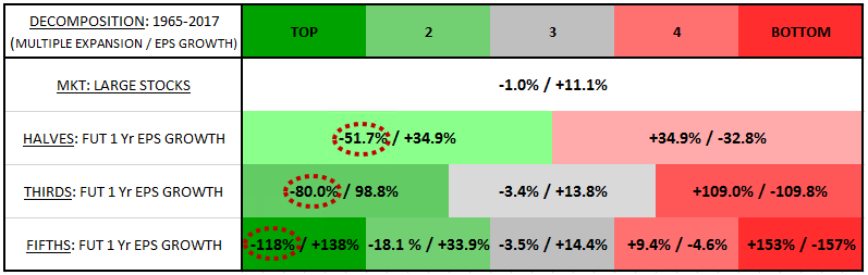
Notice the enormous multiple contraction that takes place in the top growth bins of the market: -51.7%, -80.0%, and -118% for the top half, top third and top fifth bins respectively. This contraction occurs because the stocks are experiencing rapid earnings growth, and the growth is outpacing the price increases. The contraction is orders of magnitude larger than the contraction that we saw in the corresponding growth bins of the value factor: 0.0%, -4.3%, and -9.3% for the top half, top third, and top fifth bins, respectively (see earlier table). A key reason for the difference is that the top-growing stocks in the value factor are experiencing greater price increases alongside their growth, which translates into less multiple contraction. They're getting credit for their pre-existing cheapness, the result of a previous pessimism that now has to adjust upwards.
Ultimately, when we build a bin consisting only of value stocks with the strongest future one year EPS growth outcomes, we're engaging in a form of selection bias. We're effectively gathering all of the companies in the value factor that are going to experience the good kind of multiple contraction--i.e., the kind in which the "E" will rise rapidly over the one year holding period--and putting them in the same place, inside the same portfolio. Similarly, we're throwing out all of the companies in the value factor that would go on to experience the bad kind of multiple expansion--i.e., the kind driven by one year earnings drops. What we're left with, then, is an artificially selected mix of the good kind of multiple contraction and the good kind of multiple expansion. This mix effectively cancels out, leaving the top growth bins with only a minimal net change in the multiple--a slight contraction, to be exact.
Now, the fact that the multiples of value stocks in the top growth bins contract by small amounts doesn't mean that upward re-ratings aren't taking place in those stocks. To the contrary, enormous upward re-ratings are taking place in them, far greater than the re-ratings that are taking place in stocks in the middle and lower growth bins. The market is initially pricing the stocks for earnings weakness and is instead seeing earnings strength--a 180 degree discrepancy relative to its expectations. The massive upward adjustment brought about by this discrepancy shows up in the out-of-this-world returns that the stocks go on to generate.
If we want to see multiple expansion show up in the top growth bins, all we need to do is change how we define the bins. Instead of defining the bins based on future one year earnings growth, which explicitly selects for multiple contraction in the higher growth bins, we can instead define the bins based on earnings growth over longer horizons. If, as we have argued, the market looks to the long-term when it re-rates value stocks, then we should expect the return differentials to be just as strong when the growth bins are defined on those horizons.
In the table below, we show the returns of the value factor separated into bins based on future EPS growth over the subsequent five-year period. Note that the holding period of the strategy remains one year, but we are no longer defining bin membership based on earnings growth over that year. Instead, we're defining bin membership based on cumulative earnings growth over the next five years:
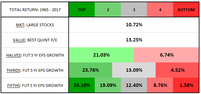
As predicted, the returns of the top growth bins on this new five-year growth definition end up being just as strong as they were on the previous one year growth definition, confirming that the market is looking to the long-term when it re-rates value stocks.
The following table shows the annual returns of the different growth bins decomposed into average contributions from holding period multiple expansion (left) and holding period EPS growth (right):
Interestingly, the top growth bins now show strong average multiple expansion, in clear contrast to the multiple contraction that we saw earlier when the top growth bins were defined on one year earnings. This multiple expansion shows up clearly in a chart of the EPS. The top growth bins exhibit the classic sawtooth pattern associated with multiple expansion, where the earnings jump upward on the rebalancing dates (vertical gridlines):
The reason that we now see multiple expansion in the top bins is that we're no longer explicitly selecting for strong future one-year growth in those bins. Instead, we're selecting for strong future five-year growth. Many stocks with strong future five-year growth experience weak growth during the first year, evidenced by the flattish to negative holding period growth shown in the decomposition. The top fifth growth bin, for example, sees growth of only +0.8% during the holding period, with the top third and top half growth bins only seeing -1.1% and -2.7%, respectively--all well below the market rate of 10%. This weak growth does not impair the returns, of course, because the market is not focused on one-year outcomes. It's focused on the long-term. As the holding period unfolds, it comes to realize that the long-term for these companies is going to be very good. It therefore raises their prices, even as their current earnings remain unchanged. The result is multiple expansion.
It's useful to stop and reflect on the wisdom that the market is demonstrating in this exercise. As the experimenters, we ourselves already know with certainty which stocks are going to have the strongest growth over the next five years. But when the market prices the stocks in real-time, it doesn't directly know that. All it directly knows is that the current earnings of the stocks are coming in weak, below the market growth rate. Still, it's able to read the tea leaves on the underlying companies and accurately detect the strong future earnings that they are eventually going to generate. It's able to look past the current weakness and correctly price the value of those future earnings in the form of multiple expansion today, delivering a return to investors today, a full five years before the actual fundamental outcome gets set in stone.