Upside-Down Markets: Profits, Inflation and Equity Valuation in Fiscal Policy Regimes
By Jesse Livermore+
September 2020
An upside-down market is a market in which good news functions as bad news and bad news functions as good news. The force that turns markets upside-down is policy. News, good or bad, triggers a countervailing policy response with effects that outweigh the original implications of the news itself.
Most investors are familiar with upside-down markets as they exist in the context of monetary policy. Bad news can function as good news in a monetary policy context because it can cause central banks to lower interest rates. If the boost from lower interest rates outweighs the negative implications of the news itself, then the overall effect on the market can be positive.
Unfortunately, monetary policy is limited in what it can accomplish as a form of stimulus. It therefore offers a weak foundation for upside-down markets. We can celebrate economic problems as catalysts for interest rate cuts, but the cuts won't usually avert the problems, at least not in full. They may buoy stock prices through portfolio preference channels, but the damage to fundamentals will tend to outweigh the buoyancy.
Fiscal policy is an entirely different matter. If deployed in sufficient quantities, it can achieve any nominal level of spending or income that it wants. When policymakers commit to using it alongside monetary policy to achieve desired economic outcomes, markets have solid reasons to turn upside-down.
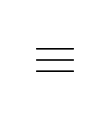
To illustrate with a concrete example, imagine a policy regime in which U.S. congressional lawmakers, acting with the support of the Federal Reserve ("Fed"), set a 5% nominal growth target for the U.S. economy. They pledge to do "whatever it takes" from a fiscal perspective to reach that target, including driving up the inflation rate, if the economy's real growth rate fails to keep up. Suppose that under this policy regime, the economy gets hit with a contagious, lethal, incurable virus that forces everyone to aggressively socially distance, not just for several months, but forever. The emergence of such a virus would obviously be terrible news for humanity. But would it be terrible news for stock prices?
The virus would force the economy to undertake a permanent reorganization away from activities that involve close human contact and towards activities that are compatible with social distancing. Economically, the reorganization would be excruciating, bringing about enormous levels of unemployment and bankruptcy. But remember that Congress is in-play. To reach its promised 5% nominal growth target, it would inject massive amounts of fiscal stimulus into the economy—whatever amount is needed to ensure that this year's spending exceeds last year's spending by the targeted 5%. To support the effort, the Fed would cut interest rates to zero, or maybe even below zero, provoking a buying frenzy among investors seeking to escape the guaranteed losses of cash positions.
The interest rate cuts, possibly into negative territory, would make stocks more attractive relative to cash and bonds. Additionally, the massive issuance of new government securities to fund the spending would shrink the relative supply of equity in the system, making stocks more scarce as growth-linked assets. Finally, the virus would give corporations financial cover to cut unnecessary labor expenses, allowing them to capitalize on any untapped sources of productivity that might be embedded in their operations. This action, which takes income away from households, would normally come back to hurt the corporate sector in the form of declining demand and declining revenue. But if the government is using fiscal policy to achieve a nominal growth target, then there won't be any income or revenue declines in aggregate. The government will inject whatever amount of fiscal stimulus it needs to inject in order to keep aggregate incomes and revenues growing on target, accepting inflation as a substitute for real growth where necessary.1
If you are a diversified equity investor in this scenario, you will end up with a windfall on all fronts. Your equity holdings will be more attractive from a relative yield perspective, more scarce from a supply perspective, and more profitable from an earnings perspective. The bad news won't just be good news, it will be fantastic news, as twisted as that might sound.
It may seem strange to think that stocks could benefit from bad news, but other asset classes that offer insured income streams, such as government bonds, behave that way. If the government is effectively insuring the income streams of the aggregate corporate sector, why shouldn't a diversified portfolio of stocks behave in the same way?
To be clear, the upside-down situation that I've described here is not the situation that we're currently in. From a policy perspective, legislators and central bankers have not implemented a nominal growth targeting regime, and the policy hawks that would normally serve as obstacles to such a regime have not yet been run out of town. But people on both sides of the aisle are increasingly coming to realize that fiscal policy is the "cheat code" of economics. If you're willing to tolerate inflation risk, you can use it to achieve any nominal outcome that you want. As people become more aware of this fact, they're going to increasingly challenge traditional approaches, demanding that fiscal policy be used to safeguard expansions and eliminate downturns. Upside-down markets will then become the norm.
In this piece, I'm going to explore the dynamics of upside-down markets, focusing specifically on the current market, which is on the verge of being turned upside-down by the unexpectedly strong fiscal response to the COVID-19 pandemic. I'm going to analyze the effects that this response—roughly $7.5T (35% of GNP) in projected deficit spending over the next two years2—will have on three variables of interest to investors: (1) Corporate Profits, (2) Inflation and (3) Equity Market Valuation.
Each variable will be treated in its own section. Topics covered will include:
(1) Corporate Profits: A derivation of a modified version of the Kalecki-Levy profit equation, a graphing of each of the equation's terms over the course of U.S. economic history, a tentative forecast of the likely trajectory of corporate profits in the current environment using past trends in those terms as a guide, and a description of the paradoxical path through which future bad news could cause profits to rise.
(2) Inflation: A description of the causes of inflation, a discussion of the ways in which expansionary fiscal policy can induce inflation and turn markets upside-down, and a quantitative estimate of the potential inflationary impacts of the government's monetary and fiscal responses to COVID-19.
(3) Equity Market Valuation: A description of the financial market impacts of fiscal policy, a discussion of the relevance of attempted buying and selling flow and the like-for-like rule, an overview of the current state of asset supply in the United States, Europe and Japan, a discussion of the upside-down portfolio effects of the COVID-19 deficits, to include an estimate of the price level and valuation that the S&P 500 would have to rise to in order to restore average equity allocations to pre-pandemic levels.
Right now, there's a bullish asymmetry in the potential for an upside-down dynamic to take hold. If things get worse, the economy will probably get more fiscal stimulus—potentially an unlimited amount, pending the outcome of the upcoming election. But if things get better, the Fed is not going to immediately tighten. Instead, the Fed is going to wait until it sees persistent demand-driven inflation above 2%—an outcome that could be difficult to achieve, particularly if inflation is measured on a core PCE basis. Of course, the investment community has already sniffed out this bullish asymmetry; it's one of the main reasons why the market has been able to set aside the ongoing uncertainties of the COVID-19 pandemic and trade its way back to all-time highs.
But the bullish asymmetry won't last forever. If we push hard enough on the fiscal side, we will eventually see inflation assert itself as a problem, causing a shift in the Fed's biases that brings the downside potential of an upside-down dynamic back into play. With markets trading near record valuations, the potential losses associated with such a dynamic could end up being quite significant.
Before moving on to the piece itself, I want to confess that it's very long—more than 40,000 words. I've tried not to waste space in it, but its length has nonetheless grown, mostly out of efforts to make its content as clear and precise as possible, and also because I've continued to push out its boundaries, using it as an excuse to lay out ideas and techniques that I find interesting. At this point, the piece is actually several stand-alone pieces merged together. If you're short on time, please feel free to skim the sections for charts and tables, using the links above to navigate to areas that you find interesting.
SECTION 1: CORPORATE PROFITS
Fiscal stimulus works through the power of government deficits. The government puts more income into the economy through spending than it takes out through taxation, causing aggregate income to rise. Corporate profit is a form of income and therefore tends to increase through this process.
The precise analytic relationship between government deficits and corporate profits is captured in the Kalecki-Levy profit equation, an accounting identity originally articulated by the economist Jerome Levy in 1908. A modified version of the equation is shown below:
(1) Corporate Profit = Corporate Investment + Dividends + Current Account Balance + Government Deficit Spending + Household Deficit Spending
Without context, the equation can be difficult to intuitively grasp, so I'm going to build it out from a set of definitions and principles. I'm then going to graph its individual terms over the course of U.S. economic history, using profit trends observed in past fiscal expansions to estimate the likely trajectory of profits in the current fiscal expansion. Finally, I'm going to use the equation to explain the paradoxical impact that bad news can have on profits in an upside-down market.
Deriving The Kalecki-Levy Profit Equation
We can think of an economy as a collection of entities that exchange goods and services with each other. The exchanges are tracked through the earning and spending of money. When you deliver desired goods and services to others, money gets paid to you. When others deliver desired goods and services to you, you give the money back. Crucially, the spending of each entity in the system gives rise to the income of other entities, which, when spent, gives rise to the income of yet other entities, and so on in complex interconnected cycles of exchange.
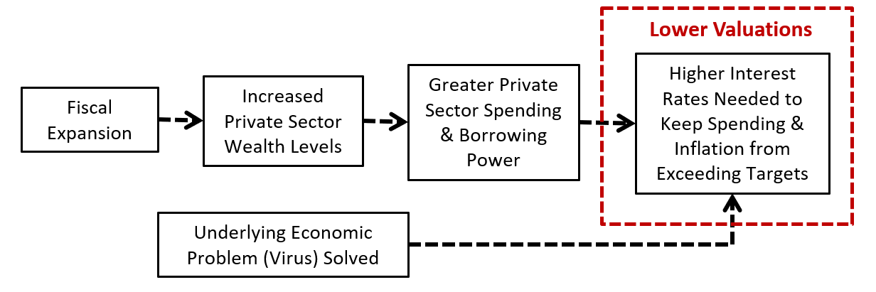
To simplify, we can separate the entities in this process into three core sectors: households, corporations, and the government. As aggregate entities, these sectors interact with each other in the way described above. Each sector receives income from other sectors in exchange for the value that it adds, and each sector spends that income back into other sectors to get that value back. The chart below illustrates the flows:
The fact that the income of each entity in the system arises out of the spending of other entities introduces a potential problem. As self-interested entities, households have a natural desire to "save", i.e., increase their "wealth" over time, which includes the real property that they own and the financial claims that they've accumulated on the system.3 The easiest way for them to save is for them to withhold some of their income from the process, i.e., not spend it back into the system after they receive it. When they withhold their income in this way, their accumulated claims on the system increase and they become wealthier. The problem, however, is that other entities in the system, including other households, lose the income that the withheld spending would have otherwise turned into. Unless those entities are willing to borrow, sell assets, or drawdown on previously withheld income, they will have to reduce their own spending, which will reduce the income of other participants down the line, and so on in a vicious cycle.
To sustain the flow of income through the system, households need to save their income in a way that also entails spending that income. Intuitively, it may not seem possible to save income and spend it at the same time, but that's only because we wrongly equate spending with consumption. When people spend their income on consumption, they use up what they've spent, so if they want to grow their wealth over time, they have to set aside a portion of their income and not spend it in that way. But there's another way they can spend it: by investing it. Investment is a type of spending that is also a type of saving; it solves the problem.
As used here, the term investment has a very specific meaning. It means the creation of a new asset, something with lasting economic value. When people earn income and invest it, their wealth grows because they gain the new asset. In funding the creation of that asset, they spend the income that they're seeking to save, transferring it to other entities in the economy. In this way, they're able to grow their accumulated wealth while also supporting the income and wealth of others.
For an illustration, consider the most common household investment—a home. When a household sets aside a portion of its income and uses the income to fund the construction or improvement of a home, its wealth grows because it converts a portion of its income into something with lasting economic value, as opposed to something that gets quickly used up. The incomes of other entities in the system are maintained during the process because the household spends the underlying money in the process of saving it. The household pays the money to the architects that design the home, the laborers that build it, and so on, creating income for those other entities.
To be clear, the term investment, as we're using it here, does not mean buying an existing asset from someone else—e.g., an existing share of stock in a company, an existing home, an existing factory, etc. When you do that, all that you're doing is swapping places with someone else in the system—that person is taking your money, and you're taking that person's shares (or their home, or their factory). Unless that person saves the money in a way that creates income for others, it will be taken out of the system with the same effect as if you had taken it out yourself.
To formalize these distinctions, we can list three things that a person can do with his or her income:
(a) Consume (spend without saving): A person can consume the income, spending it in a way that does not leave behind any value. Consumption is a way of spending without saving.
(b) Invest (spend and save at the same time): A person can invest the income, using it to fund the creation of a new asset. Investment is a way of spending while also saving. It represents a positive-sum game for the overall system. The investor gains by acquiring a new asset, and others gain by receiving the income that the investor spends in the process. The economy gains because it ends up with more assets, more wealth.
(c) Withhold (save without spending): A person can withhold the income, removing it from circulation. Withholding is a way of saving without spending. In contrast to investing, it represents a zero-sum game for the overall system. Any increase that you experience in your wealth by withholding your income will necessarily come at the expense of the person to whom your income would have otherwise gone, had it been spent.
To withhold is to receive more income than you spend, and therefore the opposite of withholding is to spend more income than you receive, i.e., to Deficit Spend. Deficit spending can be for consumption, which will lead to a reduction in current wealth, or for investment, which will leave current wealth unchanged (given that you will gain an asset in exchange for the deficit you incur). Deficit spending can be funded with money previously withheld, money obtained through the sale of current wealth, money obtained by borrowing against current wealth, or, in the case of the government, newly created or "printed" money.
Returning to the Kalecki-Levy profit equation, the starting point for the equation is the simple insight that there are two ways to save—by investing and by withholding. The total quantity saved is the sum of the two:
(2) Saving = Investment + Withholding
As explained above, withholding is a zero-sum game--one person can only do it if someone does the opposite of it. For the aggregate economy, total withholding must therefore be zero:
(3) Withholding = 0
For the aggregate economy, it follows that saving equals investment:
(4) Saving = Investment + Withholding (0)
We refer to (4) as the saving-investment identity. This identity reflects the insight that the only way that an economy, in aggregate, can "save", i.e., grow its wealth over time, is by investing its income, i.e., using that income to fund the creation of new wealth. If an economy attempts to save by investing its income, the investment will increase overall wealth in the system while preserving the flow of income through the system. But if an economy attempts to save by withholding its income, it will run into a dead-end. No new wealth will be created, and each person's attempt to withhold income will occur at the direct expense of the income of others who are attempting to do the same thing.
To illustrate this point in data, consider the table below, which shows the actual saving, investment and withholding behaviors of the U.S. household, corporate and government sectors for calendar year 1959.4 The data are taken from the National Income and Products Account (NIPA) published by the Bureau of Economic Analysis (BEA):
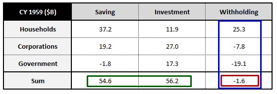
To understand the terms in the table, imagine that each sector starts the year with a certain amount of wealth. Its participants then engage in cycles of income generation and spending that track the production, exchange, and consumption of goods and services. The "saving" of each sector, shown in the second column, is simply the increase in wealth that the sector experiences over the course of the year.5 The "investment" of each sector, shown in the third column, is the amount of money that the sector deploys into the creation of new assets during the year, net of depreciation. The "withholding" of each sector, shown in the fourth column, is the amount of income that the sector fails to spend during the year.
For the year 1959, households saved $37.2B. Of that saving, $11.9B occurred in the form of investment and $25.3B occurred in the form of withholding. Withholding is a zero-sum game, so the fact that households successfully withheld $25.3B means that corporations and the government, as a group, must have negatively withheld—i.e., deficit spent—that same amount. In examining the table, we see that this is exactly what they did. As indicated in the blue box, corporations withheld negative $7.8B and the government withheld negative $19.1B. The sum comes out to negative $26.9B, a near perfect offset to the household sector's $25.3B of positive withholding. The total withholding for the overall economy, captured in the red box, was roughly zero, consistent with (3) above.
The data also confirms the saving-investment identity expressed in (4). As indicated in the green box, the aggregate saving of $54.6B is roughly the same as the aggregate investment of $56.2B. BEA data collection is not perfect, but if it had been, and if there had been no other contributors to the process, then the numbers would have been exactly the same.
In the above analysis, we ignored the impact of the foreign sector. The foreign sector can withhold against a nation's economy by receiving more income from the international trade process than it sends back through that process. Total withholding including the foreign sector must be zero, so if the foreign sector positively withholds, then the economy will have to negatively withhold, i.e., deficit spend, to make up the difference. This constraint is reflected in the chart below, which shows the annual historical withholding of the household, corporate and government sectors of the U.S. economy alongside the withholding of the foreign sector from 1929 through 2019:
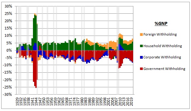
As you can see, the sum total of the withholding from all of the sectors is almost exactly zero in every year. In the case of the U.S., the government and the corporate sector tend to negatively withhold, i.e., deficit spend. Their deficit spending injects money and debt securities—financial wealth—into the household and foreign sectors, which those sectors positively withhold.
In examining the chart, it's important to recognize that withholding is not always a choice. In situations where deficit spending is occurring, it's a forced outcome. When a given sector or entity engages in deficit spending, whether through borrowing, money printing or the drawing down of past income withholdings, it injects financial wealth into the rest of the system. Someone in the rest of the system has to hold—i.e., "withhold"—that wealth at all times.
To illustrate with an example, when the government engages in deficit spending through traditional borrowing, two private sector entities are affected: (1) the person that lends to the government and (2) the person that receives the associated government spending as income. The lender trades cash for a bond of equal value and is left with an unchanged wealth position. The spending recipient, in contrast, ends up with income, new wealth to his or her name. That person might spend the income, creating income for another person, who might spend it, creating income for yet another person, who might spend it, and so on. Each person can decline to withhold the income, choosing to spend it into the coffers of someone else, but if we stop the clock on the process at a given time to collect data, we're going to find that someone is holding it at that time, having yet to spend it. That person will show up as having "withheld" it—not necessarily by choice, but by necessity, given that deficit spending took place.6
The rules governing deficit spending and withholding, then, are as follows:
Injection: Deficit spending on the part of a given entity injects financial wealth into the rest of the system.
Removal: Withholding on the part of a given entity removes financial wealth from the rest of the system.
Logically, whatever is injected by one entity has to be removed (i.e., received) by another. Whatever is removed by one entity has to be injected (i.e., provided) by another. In that sense, deficit spending forces withholding to occur, and withholding forces deficit spending to occur. Neither can occur without the other occurring.
Economically, the question that matters is: when a given entity injects financial wealth into the rest of the system through deficit spending, how much additional spending does the injection generate in the process of being withheld? Again, the wealth has to be withheld, but the process through which it gets withheld can entail significant chains of spending from person to person, entity to entity. We refer to these chains as instances of multiplication—a.k.a., "the Keynesian multiplier effect."
The same question can be posed in reverse: when a given entity removes financial wealth from the rest of the system through withholding, how much existing spending will be destroyed before someone finally deficit-spends to make up the difference? Again, someone will have to deficit-spend, but the process through which the deficit spending gets elicited could entail significant reductions in spending by people who do not want to deficit-spend. You might decide not to spend your income, taking income away from others and forcing them to either deficit-spend or cut back on their own spending. If they choose to cut back on their own spending, then they will have done what you just did, propagating the same outcome further down the system. A single reduction in spending will have then destroyed multiple instances of existing spending. We refer to this destruction as negative multiplication. It represents the opposite of the Keynesian multiplier effect.
Returning to the saving-investment identity, we can center the identity on the domestic economy by subtracting out the saving that an economy accomplishes by running a trade surplus on the foreign sector. This saving is captured in the current account balance. Adjusting (4), we get:
(5) Saving - Current Account Balance = Domestic Investment
What (5) is saying is that any aggregate saving that an economy's households, corporations and government engage in that is not accomplished by running a surplus on the rest of the world must be accomplished through domestic investment.7
Now, the saving term is just the saving of the household sector plus the saving of the corporate sector plus the saving of the government sector. We can therefore rewrite (6) as:
(6) (Household Saving + Corporate Saving + Government Saving) - Current Account Balance = Domestic Investment
Corporate saving is simply retained earnings, i.e., corporate profit (after taxes) minus the dividends that corporations pay out. Substituting, we get:
(7) Household Saving + (Corporate Profit - Dividends) + Government Saving - Current Account Balance = Domestic Investment
Rearranging the terms so that corporate profit is on the left side, with everything else on the right side, we arrive at the Kalecki-Levy equation in its traditional form:
(8) Corporate Profit = Domestic Investment + Dividends + Current Account Balance - Household Saving - Government Saving
We can make the equation more useful and intuitive by taking it a few steps further. The investment term is the sum of household investment (e.g., building new homes), corporate investment (e.g., building new factories), and government investment (e.g., building new warships).8 We can therefore rewrite the equation as:
(9) Corporate Profit = (Household Investment + Corporate Investment + Government Investment) + Dividends + Current Account Balance - Household Saving - Government Saving
Now, the saving of each individual sector is simply the sum of what it saves by investing and what it saves by withholding:
(10) Saving = Investing + Withholding (for an individual sector)
Substituting (10) into (9) for households and the government, we get:
(11) Corporate Profit = Household Investment + Corporate Investment + Government Investment + Dividends + Current Account Balance - (Household Investment + Household Withholding) - (Government Investment + Government Withholding).
The household investment term shows up as a positive and a negative--it therefore cancels out. The government investment term cancels out in the same way.
(12) Corporate Profit = Household Investment + Corporate Investment + Government Investment + Dividends + Current Account Balance - (Household Investment + Household Withholding) - (Government Investment + Government Withholding).
We end up with:
(13) Corporate Profit = Corporate Investment + Dividends + Current Account Balance - Household Withholding - Government Withholding
Now, in the case of the government, the withholding is normally negative, meaning that the government normally spends more money than it receives through taxation. To fund the difference, it either borrows money or prints money—from a fiscal perspective, these actions are effectively the same. We can therefore rewrite the negative government withholding term as a positive government deficit spending term. We can make the same change for households, replacing their negative withholding term with a positive deficit spending term. We end up with the modified version of the equation presented at the outset of the piece:
(14) Corporate Profit = Corporate Investment + Dividends + Current Account Balance + Government Deficit Spending + Household Deficit Spending
This modification offers two benefits over the original version. First, it transforms the terms so that they are all positive. It therefore allows us to represent the end result, corporate profits, as a stacked sum of quantities on a graph. Second, the modification simplifies the investment term down to the investment of one sector—the corporate sector. When analyzing corporate profits, the investment of the corporate sector is the only type of investment that we need to pay attention to. Corporate profits don't care how households and the government spend money—i.e., whether they spend it on investment or on consumption. As long as the money gets spent, the profit that corporations receive ends up being the same. The modified equation reflects this fact.
It's important to clarify that the equation is not a causal theory. It doesn't tell us anything about the microeconomic drivers of corporate profitability—e.g., supply, demand, competition, pricing power, etc. Instead, it's a macroeconomic accounting identity that holds true by definition. We can think of it as telling us that (1) financial wealth that gets injected through deficit spending ends up landing somewhere, on someone's balance sheet and (2) financial wealth that gets removed through withholding ends up being taken from somewhere, from someone's balance sheet. The equation tracks where financial wealth ends up landing and where it ends up being taken from, focusing specifically on the outcome for the corporate sector.
For those with lingering questions as to how the equation works, I've written up an intuitive description of the dynamics of each term below. Feel free to skip past the description if the dynamics are already sufficiently clear to you:
(a) Corporate Investment: One corporation's investment represents spending that becomes the revenue, and therefore the profit, of another corporation. On a net basis, this spending is not treated as a cost to the original corporation, and therefore it does not subtract from the original corporation's profit. But it adds to the profit of the receiving corporation. Aggregate profit for the overall corporate sector therefore rises as a consequence of the investment.
Now, in addition to profit, a portion of corporate investment spending will become wages and taxes for households and the government, respectively. But if these sectors are maintaining a constant withholding (i.e., if we are keeping their terms in the equation unchanged), then the implication is that they are spending the associated money back into the corporate sector. It follows that, with the other terms in the equation held constant, overall corporate profit will increase by the exact amount of any increase in corporate investment.
(b) Dividends: Dividends represent income paid by corporations to the households that own them. Importantly, these payments are not costs to the corporation. They're simply changes in the ways in which the owners of the corporations hold the underlying wealth. Before payment, the owners hold the wealth as money inside the companies; after payment, they hold it as money in their own accounts.9
If households keep their withholding constant while the corporate sector increases the dividends that it pays to them, the implication is that households are spending that dividend back into the corporate sector, either on consumption or on investment. The same is true for taxes that get extracted in the process—if the government keeps its withholding constant amid the increased income that it receives from taxes on the dividends, the implication is that the government is spending those taxes back into the corporate sector. In either case, if the other terms in the equation are held constant, any increase in the dividends that the corporate sector pays will end up back in the corporate sector as an increase in profit.
(c) Current Account Balance: Simplistically, we can say that the corporate sector earns more when it sells more abroad. A higher current account balance therefore implies higher corporate profits. More precisely and accurately, we can say that the current account balance represents a form of saving that has to show up somewhere, as a wealth gain for someone. If the other terms in the equation all remain constant as the current account balance rises, the implication is that the wealth gain is accruing to corporations, showing up as corporate profit.
(d) Government and Household Deficit Spending: If households or the government deficit spend into the corporate sector, the associated spending will show up as increased revenue and increased profit. Some of the revenue will go back to households in the form of wages and back to the government in the form of taxes, but again, assuming that the associated income is not withheld (which would change other terms in the equation), then it will be spent back into the corporate sector, where it will show up as profit. Similarly, if households and governments deficit spend into each other's coffers, and if they do not withhold the income injected by the spending, then the implication is that they are spending the income back into the corporate sector, where it will again show up as profit.
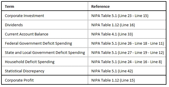
We can empirically verify the accuracy of the equation using historical NIPA data. The table below lists the specific NIPA tables and line items that quantify each term. Note that all terms are shown on a net basis—net of depreciation, taxes, and so on:
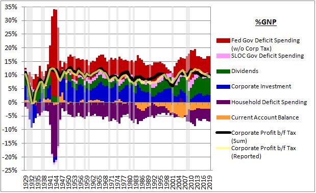
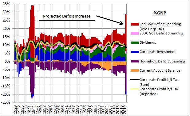
The chart below tracks the terms in the equation from 1929 through 2019, with each term expressed as a percentage of Gross National Product (NIPA Table 1.7.5, Line 4).10 If the equation is correct, then corporate profit should equal the sum of each term:
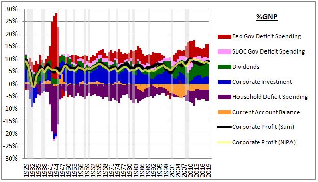
The sum of the terms is shown as the black line and the actual reported corporate profit, published by NIPA, is shown as the yellow line (both as percentages of GNP). As you can see, the two lines track each other very closely, about as closely as one can reasonably expect for a real-world data collection process that covers such a large scale. The BEA publishes a statistical discrepancy term that captures measurement error in the data collection process. If that term is subtracted from the black line, the match with the yellow line becomes exact.
Notice that the household deficit spending term, shown in purple, is almost always negative. The negative sign indicates that households positively withhold a portion of their income each year. Households are significantly more inclined to positively withhold income than other sectors because they are the only sector that consists of actual people. As actual people, they have legitimate reasons for seeking to grow wealth—they benefit from the increased security, stability, optionality, and status that additional wealth brings. The other sectors—corporations and the government—are not actual people, but rather constructs that exist to serve people. Their withholding and deficit spending decisions are not based on self-interest, but on the specific interests of the households that own them and elect them.
Why do households save by withholding? Why don't they save by investing? Because opportunities for them to save by investing—for example, by starting new businesses—aren't always practical or attractive from a risk-reward standpoint. To deliver attractive returns, new investment has to be beneficial to the economy relative to its costs. But it isn't always beneficial, and it doesn't magically become beneficial simply because households want to save.11
Returning to the chart, notice that the government deficit spending term, shown in red, is almost always positive. It has to be positive to offset the consistent positive withholding that the aggregate household sector engages in. As emphasized earlier, withholding on the part of one entity in the system requires deficit spending on the part of another. In practice, the entity that deficit-spends to make household withholding possible is the government.
If households and corporations were to deficit spend in the way that the government deficit spends, they would eventually run up against liquidity and solvency constraints. But a sovereign government is not subject to those constraints. Through its central bank, it decides the interest rate at which it borrows. And it doesn't even need to borrow—it can finance spending by printing new money. As long as there are economic participants willing to withhold the new money, and as long as the economy has the productive capacity to fulfill any additional spending that the withholding process might give rise to, economic problems such as inflation need not emerge.
This insight, most notably attributable to the British economist Abba Lerner, is a core component of Modern Monetary Theory (MMT). As the insight becomes better understood in political circles, it will increasingly drive fiscal policies that seek to guarantee desired levels of income and spending growth in the economy, policies that have the potential to turn markets upside-down, for better or worse.
Corporate Profits: Data Across History
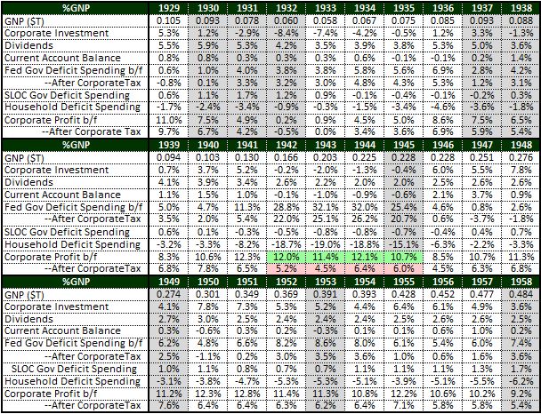
To estimate likely outcomes for corporate profits in the current environment, we can examine how the individual terms in the profit equation behaved in past environments. The table below shows each term as a percentage of GNP for each year from 1929 through 1938. Note that we separate government borrowing into Federal and State and Local (SLOC):
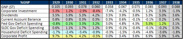
In the aftermath of the 1929 stock market crash, the U.S. economic outlook significantly deteriorated. Reduced employment and reduced income led to a substantial increase in the propensity to save, while reduced demand and reduced tolerance for risk led to a substantial decrease in the need for new investment and the willingness to undertake it. The extreme mismatch between the desire to save and the desire to invest led to a situation in which all parts of the economy attempted to withhold income at the same time. The attempted withholding caused employment and income to fall further, which caused the desire to save to become even stronger and the desire to invest to become even weaker, leading to even more attempted withholding, and so on in an imploding vacuum—the reverse of a multiplier effect.
The optimal relief valve for a destructive process of this type would be the federal government, which has the capacity to deficit spend in a way that quenches the extreme withholding demand and restores the flow of income through the system. Unfortunately, the federal government did not mount an aggressive fiscal response, and the economy continued to collapse on itself. By 1932, nominal GNP had fallen by more than 40%, unemployment was at record levels, and corporate investment and corporate profit had both fallen below zero.
Interestingly, despite the extreme amount of financial stress experienced during the period, household withholding did not appreciably rise. But that's only because it couldn't appreciably rise. Withholding is a zero-sum game, and other sectors in the economy, in particular the federal government, weren't engaging in sufficient deficit spending to make the game possible.
By the mid 1930's, the economy had returned to growth, supported by a much stronger fiscal response. However, in 1937, the introduction of new taxes, specifically the new social security payroll tax, led to a significant drop in government deficit spending. Private sector withholding demand did not fall by an amount sufficient to accommodate this drop, and the economy again entered recession. Government borrowing eventually increased to pull the economy out of recession, and by 1941, corporate investment and corporate profits were at decade highs.
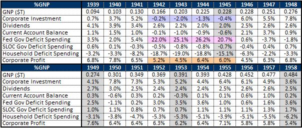
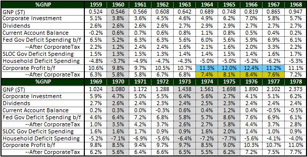
During World War II, the government engaged in an enormous amount of deficit spending to build military equipment, conduct military research, fund military operations, and pay military salaries.12 This spending led to a significant increase in all incomes, including corporate profit:
Recall that government deficit spending injects wealth into the private sector that must be withheld. In the case of World War II, the wealth that the government injected was primarily withheld by the household sector, which raised its withholding from 3.3% of GNP in 1940 to a peak of 19% in 1943. The corporate sector withheld the remainder, around 5%.
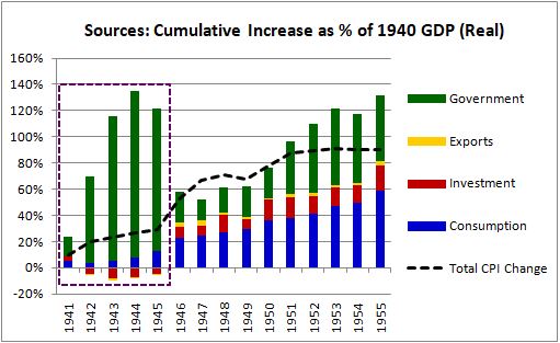
Interestingly, the government's injection was withheld by the private sector without stimulating appreciable amounts of spending, indicating a low multiplier effect. We can see this outcome in the boxed area of the chart below, which shows the cumulative change in the four sources of GDP as a percentage of 1940 GDP:
As you can see, government spending increased dramatically, but the increase did not translate into an appreciable increase in personal consumption spending or domestic investment spending. The injected wealth was quickly withheld, without jumping around in a large number of spending-turned-income-turned-spending cycles.
The lack of appreciable multiplication in response to the deficit spending was largely a forced outcome. The war production board forcibly shifted private capacity towards war production, creating domestic supply shortages. To address these shortages, goods, services, and credit were rationed. So, households didn't really have the option of spending the wealth that was being injected. They had to withhold it. Even if they had been allowed to spend it, they had good reasons not to. Those who were off fighting had little to spend it on, and those who remained at home needed to build up savings, given the uncertainty of who would return.
There's a loose analogy in this respect to the coronavirus pandemic, where government borrowing has significantly boosted aggregate household income relative to what it would have otherwise fallen to. As in World War II, the financial wealth injected through this boost is likely to be withheld by households without appreciably multiplying in spending, first because the fragile employment environment has dampened household confidence, and second because households have had to take measures to avoid contracting and spreading the virus. These measures have reduced or eliminated a substantial number of activities that households would have otherwise spent money on—group outings, vacations, sporting events, etc.
The increase in household withholding is already evident in the data. Using the personal saving rate as a proxy, we see a massive jump in April, the worst period of the lockdown, followed by a partial retreat to elevated levels in May and June (source: FRED): 13
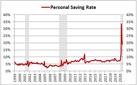
This jump has been made possible by the large government deficit, which has injected new wealth that the private sector can withhold—indeed, that the private sector must withhold.
Unsurprisingly, the jump in withholding has coincided with a sharp drop in personal consumption expenditure (PCE), shown below on a seasonally-adjusted annualized basis (source: FRED):
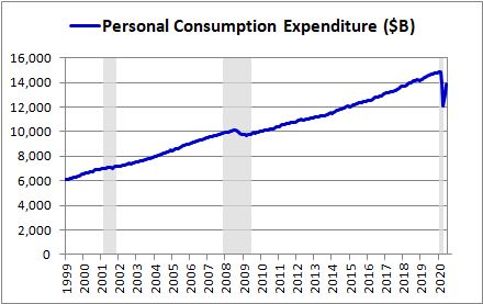
The fact that PCE dropped by such a large amount despite the stimulus confirms the severity of the impairment that the pandemic has introduced into the multiplier. While the massive injection has surely increased spending relative to the counterfactual of no injection, the increase hasn't been enough to nominally offset the contractionary impact of the pandemic itself.
The table below shows the decline in PCE by category from the January peak through the April trough (source: NIPA Table 2.4.5U). Note that these numbers are derived from seasonally-adjusted annualized rates for the individual months rather than trailing rates for the prior year:
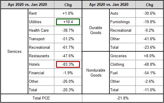
Unsurprisingly, spending on virus-impaired service industries, such as hotels, health care, recreation (e.g., gyms, live events), transportation (e.g., airlines), and restaurants suffered severe declines, while spending on goods associated with life under shelter-in-place orders, such as groceries, experienced countertrend expansions. The money to spend is there, thanks to the government's deficit spending. The problem is that it can only be spent in certain places.
In May, many parts of the economy re-opened, freeing more of the injected wealth to be spent. For perspective on the nature of the recovery in different industries, the table below shows the January-to-April declines as a percentage of total January PCE alongside April-to-June increases as a percentage of total January PCE:
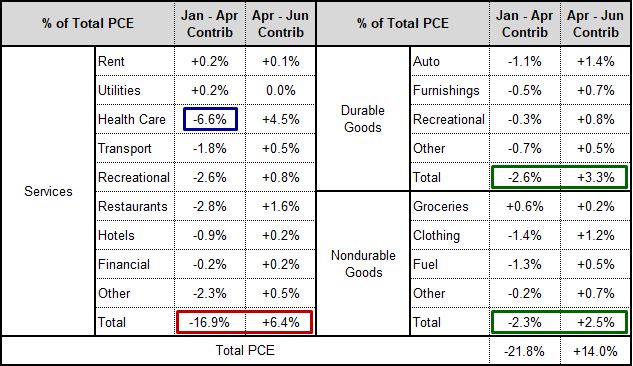
In comparing January to April, we see that the biggest negative contributor to the total PCE change was healthcare spending, which was responsible for -6.6% of the -21.8% change in total PCE. Healthcare spending is a large contributor to overall consumption spending, and it dropped significantly as patients actively avoided non-Covid-19 interactions with the medical system. During May and June, healthcare spending recovered by an amount equal to 4.5% of total January PCE, significantly less than the amount lost through April.
This incomplete recovery is mirrored across all services industries affected by the virus—recreation, restaurants, transportation, hotels, and so on. The obstacle to recovery in these industries is not demand—rather, it's the virus. The continued presence of the virus has continued to impair their ability to deliver services in ways that customers consider to be safe. No amount of stimulus is going to remove that obstacle. The threat of the virus itself has to be removed, through effective containment, convenient treatments that actually work, and ultimately, a vaccine.
Returning to the example of World War II played out, as the war played out, corporate investment fell from its pre-war levels, further offsetting the profit contribution of the government's borrowing. It fell because the economy's labor and capital resources had been forcibly redirected towards the war-fighting effort and were not available to be deployed into domestic business expansion. On a net basis, the only substantial investment that took place in the economy was government investment related to the war.
This outcome again provides a loose analogy to the coronavirus pandemic. Corporate investment is likely to drop, first as a consequence of increased corporate risk aversion related to the spike in uncertainty and the near-term shock to cash flows, and second, because many forms of investment are not practical, given virus-related concerns and constraints. We may see a redirection of corporate investment—for example, away from new commercial real estate construction towards technology supportive of remote work—but in terms of aggregate corporate investment, the sum of everything, we should expect to see a drop relative to pre-pandemic levels.
In an environment where the multiplier effect is weak, the private sector withholding that occurs in response to deficit spending will tend to preferentially occur at the location where the deficit spending is injected. The government puts income into that location through the spending and it simply stays there, without appreciably multiplying through the system. In the case of World War II, most of the spending was injected into the corporate sector, used to purchase military equipment that the defense industry was producing. On that basis, we would have expected to have seen a very large increase in corporate profit relative to other forms of income. When we look at the table, however, we see that such an increase did not actually occur. As a percentage of GNP, corporate profit peaked at roughly 5.6%, a low value by historical standards.
The primary cause of the lack of relative strength in profit during World War II was the federal government, which implemented a large excess profit tax to collect the windfall that the corporate sector was receiving. The result reflected an inversion of the principle described above: when the government takes wealth and income out of the private sector through taxation, the wealth and income losses that the private sector incurs tend to be preferentially incurred at the tax location, the place from which the wealth and income are taken. In the case of World War II, the wealth and income were preferentially taken from the corporate sector through the excess profit tax, just as they were preferentially injected into that sector through military spending. For overall profits as a share of national income, the result was largely a wash.
The excess profit tax represents a key disanalogy between World War II and the current environment. While it's conceivable that a future administration could attempt to raise the corporate tax rate to recoup some of the money currently being spent on stimulus and stabilization, the size of the tax increase is unlikely to be anywhere near the size of the wartime excess profits tax, which in some cases exceeded 90%.
To optimize the World War II analogy for this difference, we can reformulate the equation to track corporate profits on a pre-tax basis. We simply take federal corporate taxes paid and add it to both sides of the equation--to the corporate profit term on one end, reflecting what profits would have been without the excess profit tax, and to the federal government deficit spending term on the other, reflecting the additional money that the federal government would have had to borrow had the tax not been collected. We end up with the following chart:
The numbers are shown in the table below:
As you can see, the peak pre-tax profit during World War II was around 12% of GNP, more than twice the amount of the peak after-tax profit. This level of pre-tax profitability, which was 2% higher than the level seen in 2019, was among the highest levels observed in all of U.S. history.
The table below shows the values of the equation from 1959 through 1978:
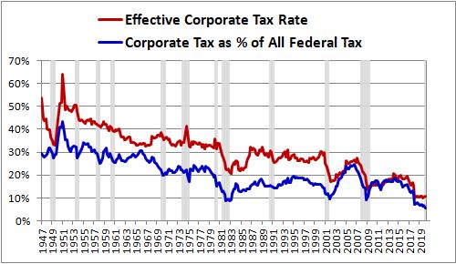
The elevated gap between pre-tax profits and after-tax profits seen during the period reflects the augmented role that corporate taxation came to play as a source of government revenue during and after the war. This role has since declined, coinciding with an increase in after-tax corporate profitability (source: FRED):
The table below shows the values of the equation from 1979 through 1998:
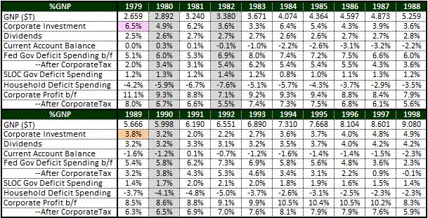
Another feature of the data worth noting is the steady decline in corporate investment that has occurred over time. At the 1979 cycle peak, corporate investment was 6.5% of GNP. Ten years later, at the 1989 cycle peak, it was only 3.8% of GNP.
We see a continued decline in the data from 1999 through the present:
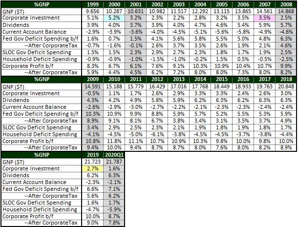
At the height of the 1999-2000 technology boom, corporate investment was 5.2% of GNP. At the height of the mid 2000's expansion, it was 3.5% of GNP. At the height of the most recent expansion, it was only 2.7% of GNP, close to a third of its value in 1979.
The declining trend in corporate investment is sometimes cited as evidence of poor corporate citizenship. In an effort to stimulate investment and job creation, legislators and policymakers have consistently given the corporate sector what it has asked for, reducing the tax, regulatory and financing burdens imposed on it. In response, it has shrunk its investment outlays and used the proceeds to pay dividends and buy back shares, expenditures that benefit shareholders and no one else.
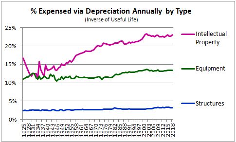
In defense of the corporate sector, we should note that a substantial portion of the decline, if not all of it, is the result of accounting conventions. Unlike GAAP, NIPA treats research and development expenses as investments, capitalizing them as intellectual property and depreciating them over an assigned useful life. The average useful life that it assigns to them (4-5 years) tends to be much shorter than the average useful lives that it assigns to traditional investments in equipment (7-8 years) and structures (25-30 years).
The chart below shows the average percentages of the net stock of different types of corporate fixed assets that were expensed via depreciation in NIPA each year from 1925 through 2018. As you can see, the percentage of intellectual property investments expensed via depreciation each year has grown over time, indicating a shrinking assigned useful life. The number is now between 20% and 25%, reflecting an assigned useful life of only four to five years (source: NIPA Fixed Asset Tables 4.1, 4.4):
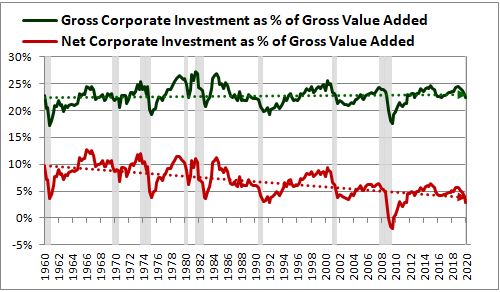
In recent decades, as corporate investment has shifted towards intellectual property and away from equipment and structures, the result has been an effective increase in the depreciation expense assigned to the same level of gross investment, causing an apparent decline in investment net of depreciation. If the shortened useful life that NIPA assigns to intellectual property investments is accurate, then the associated decline in net investment is real and should be taken seriously. But if it isn't accurate, then the decline should be ignored.14 Either way, actual gross corporate investment as a percentage of gross corporate output (value added) has not actually declined (source: NIPA Table 5.1):
If we were to reconstruct the profit equation using numbers gross of depreciation rather than net of depreciation, we would find that gross profit margins have increased significantly relative to net profit margins. Data on gross profit margins are not available for national corporations, but they're available for domestic corporations (source: NIPA Table 1.14):
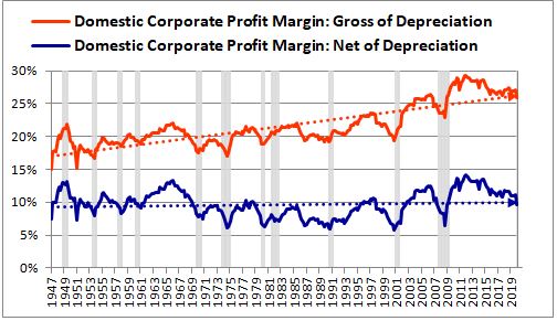
As you can see, gross profit margins, which are essentially cash flow margins, have grown dramatically relative to net profit margins. In light of this result, a critic of the corporate sector could reasonably pose the question: "Why haven't your investment outlays kept up with the enormous growth in your cash flows?" Presumably, the answer is that attractive investment opportunities have become less plentiful over time, leading corporations to instead direct their excess cash flows into dividends and share buybacks.
Forecasting Likely Profit Outcomes in the Current Environment
The deficit that the U.S. government is expected to accrue in response to the COVID-19 pandemic represents financial wealth that will be injected into the private sector. The impact that this wealth will have on corporate profits will depend on what happens to it when it gets injected. Someone in the private sector will have to withhold it—who will that be? How much spending will it trigger in the process of being withheld? The answers to these questions will depend on where the injection is delivered. A corporate tax cut, for example, is a direct injection into the corporate sector. It does not require any subsequent activity to count as profit. A household tax cut, however, will only affect profit if the proceeds get spent, directly or indirectly.
The Congressional Budget Office (CBO) estimates the current structural federal deficit to be roughly $1.1T. This deficit is the deficit that would have been incurred if the COVID-19 downturn had never happened. The additional deficit that will be incurred will originate from cyclical impacts associated with the downturn, e.g., declining tax revenues and increased transfer payments, and from the series of economic relief measures that have been implemented.15
The economic relief measures contain certain types of fiscal outlays that are clear injections into a specific sector: examples include expanded unemployment benefits and direct payments, which are direct injections into households, and tax cuts and forgiven loans, which are direct injections into corporations.16 The destinations of other types of outlays, such as funding for COVID-19 testing, are more difficult to pin down. In the table below, I've put together a very rough estimate of the likely destinations of the outlays associated with each measure:
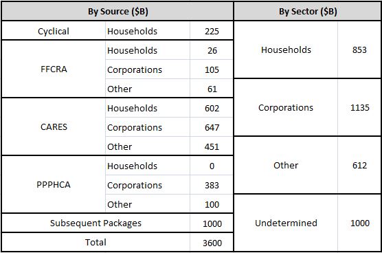
The left side separates the projected deficit into its legislative sources, while the right side shows the deficit by the expected destination of the outlay: households, corporations, and "other", which refers to entities such as state and local governments and non-profit organizations. The "unknown" category refers to outlays associated with future expected measures that have not yet been defined in legislation. Note that government loans do not constitute fiscal outlays unless defaulted on or forgiven, so the table only includes the forgivable portion of paycheck protection program (PPP) loans. We assume that the Fed will break even on the sum total of its asset purchases and direct lending activities, and therefore we exclude the collateral that the Treasury has provided to the Fed from the tally.
As you can see in the table, a significant portion of the outlays are set to go directly into the corporate sector. Some of that revenue will go to costs and some will go to profit, offsetting organic profit losses incurred in the downturn. If the offset is sufficient to quench corporate withholding demand and stimulate investment and dividend spending, then the outlays will have the potential to multiply in additional profit, assuming that the recipients of the associated income spend it back. But if the outlays aren't sufficient to quench corporate withholding demand, then they will show up as corporate withholding and nothing else—profit that sits idle on corporate balance sheets.
Similarly, if the outlays to households and other non-corporate entities are sufficient to quench the withholding demand of those entities and stimulate spending on corporate goods and services, then they will translate into additional profit for the corporate sector. But if the outlays aren't sufficient to quench the withholding demand, then they will show up as withholding and nothing else—income that sits idle on non-corporate balance sheets.
Without question, the outlays are going to exert multiplier effects on corporate profit. The question that will determine the ultimate profit outcome is whether those effects will be sufficient to offset the negative multiplier effects associated with the downturn—corporate layoffs leading to household spending reductions leading to declining profits leading to further layoffs leading to further household spending reductions and so on in a vicious cycle. With respect to that question, the most important consideration is the epidemiological consideration.
At one extreme, we can envision an optimistic scenario in which the virus naturally goes away, or in which an effective vaccine or other conclusive medical solution is expeditiously developed. All of us—including those of us who are hypochondriacs—would then be able to return to our normal behaviors without fear of getting sick. The elevated withholding demand would gradually decline, prompting households to spend and businesses to hire and invest. These improvements would be occurring while the government injects record amounts of financial wealth into the system, wealth that someone has to withhold. Given the lack of an excess profits tax, corporate profit in such a scenario could very well end up being higher than it was before the pandemic, at least from the point of recovery forward.
At the other extreme, we can envision a pessimistic scenario in which the virus continues to aggressively circulate and infect, and in which a satisfactory vaccine or other medical solution proves to be elusive. Not everyone will maintain current behavioral changes under such an outcome, but enough people probably will, forcing the economy to undertake a more painful and drawn-out restructuring of the kinds of goods and services that it's aligned to produce. The current state of fragile employment, reduced confidence, weak investment, and tepid spending would then persist. Under such a scenario, current levels of deficit spending could prove entirely insufficient to quench the private sector's increased withholding demand, leading to a significant net decline in profits.
With respect to profits in a pessimistic scenario, some have expressed concern that the presence of the virus will increase corporate operating costs. But we have to remember that one entity's "cost" is another entity's income. If the virus forces corporations to spend more in their operations, the profit impact will be determined by what the recipients of that increased spending—presumably, households, but also other corporations—do with the income created by the spending. If they withhold it, either out of preference, or out of an aversion to price increases in the areas where they would otherwise spend it, then the effect on profit could be negative. But if the recipients spend it back into the corporate sector, the effect could be a wash.
In the chart and table below, I generate a tentative 2020 NIPA profit forecast by assigning specific numbers to the terms in the equation. I apply the pre-tax version of the equation using the following conservative assumptions:
A pre-corporate-tax federal government deficit of $4.84T (consisting of an after-corporate-tax deficit of $4.7T plus $140B in corporate taxes collected), 22.3% of GNP.
A current account balance and state and local government deficit of -2.1% and 1.7% of GNP, respectively, equal to the trailing twelve-month values as of the end of the first quarter of 2020.17
Dividends of 4.7% of GNP, calculated by assigning an estimated decline equal to the decline observed in the 2009 recession.
Corporate investment of -2.0% of GNP, equal to the level seen in 1943, the year of peak war-related retrenchment. Note that investment is a net term, so a negative number indicates gross investment insufficient to offset depreciation.
Household withholding of 16.0% (i.e., household borrowing of -16.0%), equal to roughly three-quarters of the after-tax government deficit, the same ratio seen in 1943.
The black line in the chart below shows the resulting profit forecast:
The table below shows the numbers in the equation. To obtain after-tax numbers, I simply apply the effective corporate tax rate for 2019 to the pre-tax estimates:
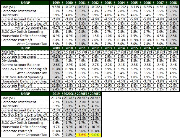
Under the stated assumptions, after-tax corporate profit drops from around 9% of GNP before the pandemic to around 7.7% of GNP after it (see 2020E1 in the table). That drop, when coupled to the CBO's estimated 2020 GNP drop of 5.6%, produces an overall profit drop of roughly 20%. Not a good outcome, but dramatically better than the Great Depression outcome that would have ensued in the absence of a strong fiscal response.
If we alter the forecast to reflect the corporate investment level observed in the 2009 recession, which is roughly the same as the level calculated using CBO's current projections, we get an after-tax profit of 9.0% of GNP (see 2020E2 in the table), the same number seen in 2019. The overall profit decline relative to 2019 ends up matching the GNP decline—a drop of only 5.6%. Such a small decline might seem unrealistic, but the enormous contribution that the government is making has left it well within the realm of possibilities.
It's important to note that these are estimates of NIPA profits, which only capture income from current production. Actual earnings numbers reported by companies in accordance with generally accepting accounting principles (GAAP) will likely contain larger downward swings, given the need to write down the values of past investments. Regardless, the important takeaway is that investors should not be surprised if corporate profits end up coming in stronger than expected for a recession as deep as this one has been—the government's actions have quite literally changed the equation.
For fundamental investors, the profit numbers that emerge for 2020 shouldn't be the focus. Equity value derives from a long-term stream of future cash flows, and 2020 is only a single year in that stream. When looking out over the long-term, the important point to remember is that the virus doesn't damage actual physical or intellectual capital—the assets that make corporations valuable. It simply prevents the public from making full use of those assets, despite otherwise wanting to. The lack of utilization is obviously a problem for corporations in that it deprives them of cash flow and exposes them to the risk of bankruptcy. But If the government, through its stimulus and liquidity provisions, can successfully bridge the system through the period of reduced utilization associated with the pandemic, then everything can eventually go back to the way it was, with the only cost being a temporary period of reduced income.
Instead of spending the wealth that the government injects through its deficits, cautious households may choose to withhold it, preventing it from turning into profit. But even if this happens, the benefit to profit will not be lost. The wealth, in being withheld, will lead to a strengthening of household balance sheets, which will free up space for households to increase their borrowing and spending in future years, causing an increase in profit that shows up with a lag. So even if the pandemic imposes a year or two of profit weakness on the corporate sector, that weakness can get recouped in the strength that follows, assuming that the actual problem—the virus—gets solved.
Profit Outcomes in an Upside-Down Market
The chart below shows year-over-year changes in the earned disposable income and consumption spending of U.S. households from January of 1960 through May of 2020.18 The upper lines (red, green—left axis) represent nominal changes and the lower lines represent real changes (blue, yellow—right axis) (source: NIPA Tables 2.4.5U and 2.6):
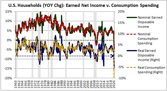
These aggregates grow together because they depend on each other: disposable incomes are the funding sources for consumption expenditures, and consumption expenditures are the revenue sources for disposable incomes. Periodically, their growth rates decline, sometimes to levels below zero.
What causes these declines?
One possible cause is policy. In order to grow, economies need certain monetary and fiscal conditions to be met—e.g., available credit at economically-viable rates, a government deficit sufficient to quench private sector withholding demand, and so on. When these conditions are challenged through policy actions, growth can fall or shift into contraction. Outside of policy, we can identify at least three additional causes of growth declines: Supply Shocks, Supply-Demand Mismatches, and Financial Wealth Contraction. We discuss each cause below:
(1) Supply Shocks: Events can occur that reduce the economy's capacity to produce goods and services that consumers want to consume. The production of those goods and services is the basis for income and spending, and therefore reductions in that capacity can lead to declines in both.
To illustrate with an extreme example, suppose that a gigantic meteor were to slam into some part of the country, destroying meaningful parts of the local economy. Everyone who earns income from those parts would lose income, and everyone who consumes goods and services produced in those parts would have fewer goods and services available to purchase and consume. If the shock proves to be inflationary, nominal levels of income and spending may remain constant. But real income and spending will necessarily fall.
(2) Supply-Demand Mismatches: Parts of the supply-side of the economy can become misaligned with the demand-side, structuring themselves to produce goods and services that are not sufficiently wanted. Alternatively, events can occur that cause the consumption preferences of the demand-side of the economy to change more rapidly than parts of the supply-side can keep up with. In both cases, income and spending growth will slow.
COVID-19 is an example of the latter case. Consumers like to eat at restaurants, go on vacations, attend live events, and so on, and the supply-side of the economy has correctly responded to those preferences by organizing itself to produce the desired supplies of those activities. Unfortunately, the ongoing presence of COVID-19 has dramatically reduced consumer demand to engage in the activities, with the result being a sharp drop in overall consumer spending. Incremental spending that would have gone into the activities has no reason to go elsewhere, so it has disappeared.
(3) Financial Wealth Contraction: The private sector has the ability to create financial wealth through credit expansion and through the pricing of assets. Sometimes, it uses these processes to create wealth that doesn't deserve to be created—wealth that isn't tied to the production of goods and services that people actually want. The destruction of this wealth, either naturally or in response to policy action, can force affected individuals to reduce their spending.
To illustrate with an extreme example, suppose that a very large segment of the population starts speculating in Bitcoin, using leverage where available. The price rises to $10,000,000, creating enormous financial wealth for millions of people. This wealth isn't real, it isn't tied to the production of goods and services that consumers actually want to spend money on, and therefore it won't be able to generate the cash flows necessary to justify its existence or service the debt on which it was built. If allowed to spill over into broader spending, it will put upward pressure on prices, driving a monetary policy response that will jeopardize the speculative fervor that is holding it together. Whether monetary policy ends up being the catalyst, or some other catalyst emerges, the system will find a way to destroy the wealth. When that happens, the unlucky people stuck holding it will be forced to reduce their spending—not because they don't want to spend, but because they can't afford to. They will have effectively given their wealth away to the people who they bought Bitcoins from.
The economic pain associated with these processes is not a mistake. It's a consequence of losses that need to be accepted and imbalances that need to be corrected. With respect to supply shocks, when the economy's productive capacity is damaged, reduced output is a given. Someone has to take the associated losses. With respect to supply-demand mismatches, if a part of the economy is producing things that people don't want, the financial squeeze that affected shareholders and employees will experience is by design—the system is asserting itself, forcing economic resources that are being inefficiently utilized to redeploy themselves in ways that meet the actual demands of the population. With respect to financial wealth contraction, if credit expansions and asset bubbles have been used to create financial wealth that is not backed by actual real wealth—the capacity to produce real things that are wanted by the economy—defaults and asset price declines are the proper remedy. The spurious wealth never should have been created and needs to be taken back.
The problem with the pain experienced in these processes is that it tends to propagate, moving well beyond its starting location. The justified losses experienced at ground zero will tend to depress income, spending and credit availability in other areas of the economy, causing losses that eventually spread everywhere through negative multiplication. As equity investors, we can use diversification to dilute away the risks associated with a single business or a single sector, but we can't use it to dilute away the risk of broader damage of this type—the risk is system-wide.
When consumption spending declines, legislators and policymakers have the ability to intervene, delivering liquidity and financial wealth to the places where it's needed. But intervening comes with costs, including: (1) unfairness and moral hazard, which can occur when people are protected from market consequences that they should have to face, (2) prevention of necessary adjustments, which can occur when the injected liquidity and financial wealth remove the stress that would otherwise force the adjustments, (3) inflation, which can occur when the liquidity and financial wealth that are injected as a remedy lead to more spending than the economy can support.
In a laissez-faire system, legislators and policymakers assign infinite weight to these costs and therefore never intervene. They leave the system alone and allow losses to negatively multiply until the damage has run its full course. If you are a diversified equity investor in a laissez-faire system, anything that causes a downturn in consumption spending will therefore represent an existential risk to you. If the downturn gives rise to a runaway contractionary process, the equity tranche of the economy will get wiped out and you will suffer extreme losses, regardless of whether you are diversified across your holdings.
The COVID-19 situation is unique in that none of the normal costs associated with intervention are present. With respect to unfairness and moral hazard, nobody did anything wrong, and therefore there's no need to worry about the implications of providing assistance. With respect to adjustment, if the problem of the virus can eventually be resolved, then there's no need for the supply-side of the economy to adjust—in fact, we don't want it to adjust, we want it to maintain the ability to produce the things that it was producing before the virus emerged, because consumers will go back to wanting those things when the virus goes away. With respect to inflation, current rates of inflation are very low and are likely to go even lower in the absence of aggressive policy action.
With these costs eliminated from the equation, it's no surprise that legislators and policymakers have responded to the pandemic by implementing the single largest stimulus intervention in history. If there were ever a worthy time to intervene, this is it.
To illustrate the effects of the COVID-19 intervention, the chart below shows U.S. household income alongside consumption spending for the months of January through June of 2020. The earned disposable income column represents all forms of household labor and capital income, to include income associated with government programs funded by the recipient. The government assistance column represents all forms of income not funded by the recipient, which includes income associated with normal and enhanced unemployment insurance, medicaid, and direct payments to households. The total disposable income line is the sum of the two columns (source: NIPA Tables 2.4.5U and 2.6):

From the January peak through the April trough, consumption spending fell precipitously, suffering a 19% contraction. This contraction coincided with a 7% contraction in earned disposable income. Total disposable income, however, grew by 14%, reflecting the enormous government assistance provided by the CARES act. The assistance was enough to turn the largest three-month income contraction in U.S. economic history into the largest three-month income expansion.
When this assistance expires, legislators will have to confront a critical set of questions. Should they renew it? If so, should the amount of assistance—in particular, the $600 per week currently being paid in enhanced unemployment benefits—remain the same? Should it be reduced? Should it be increased? These questions will be difficult for legislators to answer because the assistance was not provided as part of a well-defined, well-understood policy strategy. Legislators saw the economic pain that was being experienced and came up with an arbitrary fiscal number to inject in relief.
Before the pandemic, nominal household disposable income was growing somewhere between 4% and 5% per year. If the goal of the intervention is to avert the contraction associated with the pandemic, then a potential fiscal response that would make sense would be a response that targets that income growth rate. In deciding on assistance, legislators would examine the state of the private economy and calibrate the assistance to ensure that total household disposable income continued to grow at 4% to 5% per year.
On a year-over-year basis, earned household disposable incomes are still in contractionary territory relative to the peak. They have to be, given that significant parts of the economy remain impaired by the virus. Fiscal assistance therefore needs to be extended. The amount of assistance provided in the CARES act, however, has caused total household disposable income to significantly overshoot the normal rate, driving it up by 9% relative to the prior year. For income growth to return to the normal rate, a reduction in the amount of assistance may be needed.
We refer to a policy strategy that calibrates deficit spending to achieve a targeted income growth rate as fiscal income targeting. The strategy is not explicitly employed by any market-based economy at present, but it may be employed in the future as politicians become more comfortable with deficit spending. If you are a diversified equity investor, its implementation will significantly change the risk profile of your investments. The prospect of a broad decline in the incomes of the customers of your companies—a serious, unavoidable risk in the traditional laissez-faire framework—will disappear. Bad news won't be as bad, because it won't be able to propagate to aggregate household income. As long as the companies in your portfolio continue to produce goods and services that consumers are willing to spend money on, those companies will continue to receive the revenue that they need in order to remain profitable.
The problem with fiscal income targeting is that households aren't necessarily going to spend the income that they receive. Instead of spending it, they can choose to withhold it, which is what they've done in the current pandemic, evidenced by the 7% decline that has occurred in total consumption spending (despite a rise in total disposable income). As a diversified equity investor in a fiscal income targeting regime, you are fully exposed to the risk that households will withhold the assistance delivered to them. Bad news on the economy could therefore still be bad news for you if it causes that risk to materialize.
Instead of targeting aggregate incomes, a more aggressive approach would be to target aggregate spending. In a spending targeting regime, legislators monitor the condition of the economy and inject whatever amount of wealth they need to inject in order to ensure that nominal spending grows at the desired nominal rate—say, 5% per year. If households undermine this effort by withholding the wealth, then legislators can respond by injecting wealth with an explicit "spend by" date. Instead of issuing checks, for example, they can issue gift cards that expire. If that solution proves insufficient to stimulate spending, then they can just do the spending themselves, sending purchase orders directly into the corporate sector. Again, fiscal policy is a cheat code--when it wants to, it will always win.
A fiscal policy regime that targets aggregate spending would eliminate the main fundamental risk that diversified equity investors are exposed to: the risk of aggregate declines in corporate revenue and cash flow growth. The corporate sector would never again suffer these declines because its revenues, which track total nominal spending, would be guaranteed to grow at the rate targeted by fiscal policy. If you are an existing shareholder with a diversified portfolio that tracks the revenue growth of the overall economy19, the regime would leave you exposed to only two remaining sources of fundamental risk:
Capital Formation: You would remain exposed to the risk that new companies will form, drawing revenue away from the existing companies in your index.
Profitability: You would remain exposed to risks related to profitability, i.e., the amount of value that you manage to extract from your revenues in comparison with the value extracted by your employees, your lenders, and the governments that tax you.
Bad news for the economy would be good news for you as a shareholder because it would mitigate both of these sources. It would stunt new capital formation, which would mean fewer new companies to share the policy-controlled revenue pie with. It would boost unemployment and weaken the general bargaining position of labor, which would allow you to pay lower wages. Those lower wages would not feed back to you as lower spending and lower revenue because the government would effectively be insuring the economy's spending and revenue through the targeting, beefing up the very paychecks that you've trimmed down. You would therefore be free to squeeze out any untapped sources of productivity that might be latent in your operations, keeping the gains for yourself. If the contraction were to also provoke a monetary response in the form of interest rate reductions, your interest expense would decline, driving a further boost in your profitability.20 Finally, the likelihood of a corporate tax increase would fall as the policy bias shifts away from contractionary measures that might slow the economy down.
What I've described here is an upside-down market, where policy intervention creates a condition in which everything is the opposite of what it normally is. Investors would still be exposed to the negative effects that bad news can have on investor sentiment and appetite for risk, but fundamentally, in terms of the discounted value of future earnings, bad news would be good news.
For a concrete example of an upside-down market dynamic, imagine that a supervirus with the following characteristics were to emerge: (1) carried by mosquitos, but not damaging to them, such that it never leaves the biosystem, (2) transmissible via both human respiratory emissions and mosquito bites, (3) confounding to the human immune system, such that humans cannot build up reliable immunity to it, and (4) highly morbid, with a 5% infection fatality rate across all age groups. Given these frightening characteristics, the virus would be the equivalent of a lethal version of the common cold—something that people would be at risk of acquiring in any public outdoor setting for the rest of their lives. The only way for them to protect themselves would be to permanently lock down, doing everything from inside their homes.
Obviously, a supervirus of this kind would be devastating to the economy. It would force a restructuring of almost everything currently in place, generating extreme levels of unemployment and bankruptcy. In a traditional laissez-faire system, equity investors would get destroyed. Significant portions of their portfolios would be rendered worthless.
But in a regime that uses fiscal policy to target aggregate spending, the scenario would boost the nominal values of their portfolios, as weird as that might sound. A sufficient quantity of gift cards or other stimulus items would be continually disseminated to ensure that overall nominal spending in the economy continued to grow on target. Overall corporate revenue growth, which tracks overall spending growth, would therefore be preserved. For any company that lost revenue, some other company would gain it—revenue would go from restaurants to grocery stores, for example, as people made their own food in lieu of eating out. Diversified investors who own both the winners and the losers in this process would experience no net revenue losses. Meanwhile, profit margins would expand as the Fed cut rates, possibly into negative territory, and as millions of displaced employees found themselves in weaker bargaining positions. The end result would be higher earnings and therefore higher stock prices once investor sentiment normalized (if it ever could).
If the winning segments of the economy were bottlenecked and unable to sufficiently expand capacity, then the stimulus would generate inflation. The nominal spending target would then be achieved through the inflation, exposing equity investors to potential losses in real terms. But nominally, relative to cash in the bank, they would be clear beneficiaries.
In using a supervirus scenario to illustrate the dynamics of an upside-down market, my intention is not to suggest that the economic winners of the current virus scenario are a buy. Those winners will obviously do very well if COVID-19 remains an indefinite problem, but their current prices and valuations probably already reflect this fact. If we get a better-than-expected outcome with respect to the virus—e.g., a vaccine that works and that is able to be expeditiously distributed—their current expensiveness will become a source of risk. The companies to own will be companies that are exposed to the economic impacts of the virus and that have been priced cheaply in light of that exposure. If the risks of the virus subside, those companies will recover. The residual presence of large fiscal stimulus in the system will make their recoveries even stronger.
SECTION 2: INFLATION
In the previous section, we saw how fiscal policy regimes that target aggregate income and spending levels in an economy can create "upside-down" dynamics in which bad news functions as good news. But the United States and other developed market economies do not actually employ these regimes. Instead, they employ monetary policy regimes that target inflation. Fiscal policy is available in these regimes to provide support when political incentives align, but monetary policy remains the primary tool for achieving desired outcomes.
In this section, I'm going to explore the impact that fiscal policy can have on markets in monetary policy regimes that target inflation. I'm going to begin the section by describing the different mechanisms through which inflation can occur in an economy. I'm then going to explain how fiscal policy can trigger these mechanisms and produce upside-down dynamics. Finally, I'm going to examine the monetary and fiscal response to the COVID-19 pandemic and assess the likelihood that it will provoke significant inflationary pressure in the United States.
The Causes of Inflation
Inflation is one of the least well-understood phenomena in all of economics. The prevailing theory for how and why it occurs was developed by the British economist John Maynard Keynes. Borrowing from Keynes' framework, we can identify at least four different types of inflation: (1) cost-push, (2) demand-pull, (3) structural and (4) hyper.
Cost-Push Inflation is inflation brought about by increases in the cost of producing goods and services. An example would be a situation in which a critical commodity becomes more expensive to produce. The prices of goods and services that use the commodity will rise as the increased cost is passed through to consumers.
Demand-Pull Inflation is inflation brought about by excessive demand for goods and services. An example would be a situation in which an unproductive expansion of credit leads to a rapid rise in wealth and income that drives spending levels above the economy's capacity to produce.
Structural Inflation is inflation brought about by the expectations and commitments of economic agents. It occurs most easily in economies that have already been experiencing inflation for other reasons. As participants become accustomed to the inflation, they will come to view it as "normal", incorporating it into their economic behaviors. Sellers will become more likely to attempt periodic price increases and buyers will become more likely to accept those increases. Workers will become more likely to request periodic wage increases and employers will become more likely to grant those increases. When entering into contracts, participants will build their inflation expectations into the contracts, writing periodic price increases into the terms. These actions will produce a self-fulfilling form of inflation that continues independently of other causal sources.
Hyperinflation is inflation that results from the rejection of a currency as a store of value. It typically emerges out of a feedback loop between two mutually-reinforcing conditions: (a) Economic participants lose confidence in the future purchasing power of a currency and become unwilling to hold it, causing it to depreciate, and (b) The government issuing the currency has hard liabilities—e.g., inflation-linked debt, debt in a foreign currency, real resources that need to be purchased to fund vital causes, etc.—and is forced to issue ever-increasing amounts of the currency to fund those liabilities. The issuance deepens the loss of confidence and accelerates the depreciation, forcing additional issuance in a vicious cycle.
The chart below shows the average annual price inflation of relevant goods and services in the United States economy from May 1998 through January 2020, just before the pandemic hit (source: BLS):
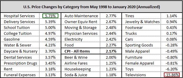
The differences in inflation seen across different goods and services is likely attributable to cost-push factors. To understand why cost-push factors would generate these differences, we need to remember that all industries depend on a common input, labor. In real terms, that input tends to become more expensive over time as employees capture the economy's overall productivity growth in their wages. For this reason, industries that aren't able to appreciably increase their productivity tend to experience above-trend inflation. They rely on a labor supply whose cost is increasing faster than inflation, but they aren't able to use that supply any more efficiently to generate output, so they have to pass the cost on to consumers, raising prices at a pace that exceeds inflation as well.
This phenomenon is known as the Baumol effect. It helps explain why industries that are prone to low productivity growth, such as higher education, have experienced above-trend inflation. Colleges are in the business of selling a prestigious credential, and one of the determinants of the prestigiousness of the credential is a low student-to-teacher ratio. In 1998, it took one professor to teach a college course at a specified student-to-teacher ratio. Today, it takes that same number, by definition. And given the increased emphasis on creating the optimal educational environment, it takes more administrative faculty working in the background. Meanwhile, the cost of attracting highly-educated people to perform teaching and administrative functions at the college level has risen at a rate that exceeds inflation. The cost of the final product—the diploma credential—has therefore risen at a rate that exceeds inflation as well.
Apart from differences in productivity growth, an additional potential cost-push contributor to the observed differences in inflation is globalization. Durable goods industries such as clothing, toy, furniture, and electronic manufacturing are more able to arbitrage differences in international labor costs than services industries such as child care that can't offshore their production as easily. As a consequence, durable goods industries have experienced less inflation, if not outright deflation.
The chart below shows the price indices of all contributors to gross domestic product (GDP) relative to the overall GDP price index from 1929 through 2019 (source: NIPA Table 1.1.9). The GDP categories are: Investment (Structures, Equipment, Intellectual Property, Residential), Personal Consumption Expenditures (Services, Durable Goods, Nondurable Goods), Government Expenditures, and Trade (Exports and Imports).
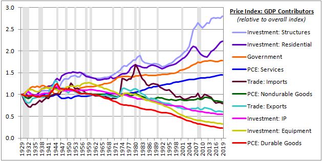
Confirming the Baumol Effect and the potential contribution of international labor cost arbitrage, durable goods, and equipment (the corporate investment equivalent of durable goods) have experienced the lowest inflation of all consumption categories and of all categories in general. They've been in outright deflation for almost three decades. Services, in contrast, have experienced the highest inflation of all personal consumption categories. They've been consistently outpacing the overall index since the end of World War II.
Interestingly, the two price indices tied to real estate—residential investment and corporate investment in structures—have experienced the highest inflation of all categories. Their relative inflation is attributable to similar Baumol-like cost-push factors. The natural scarcity of desirable land supply prevents real estate from experiencing the kind of productivity growth that other industries experience. Income drives the ability to purchase real estate, a purchase that every participant in the economy has to make, either directly through ownership or indirectly through renting. Since income grows faster than inflation over time, the cost of real estate tends to grow faster than inflation as well.
Shifting our focus to the pandemic, the chart below shows the total (not average annual) inflation of relevant goods and services in the United States during the COVID-19 pandemic (source: BLS):
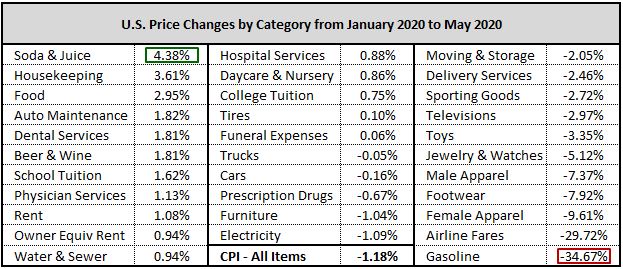
In contrast to the prior table, the observed differences in the table above are likely attributable to demand-pull factors. The prices of things that can't be consumed due to the pandemic—e.g., airline fares—have plunged, while the prices of things that now have to be consumed in greater amounts—e.g., grocery store food, since restaurants are impaired—have noticeably increased. Cost-push sources may also be contributing to the increases seen in services such as housekeeping, which are more difficult to provide in the presence of the pandemic.
When prices go up, some entity necessarily earns more income per unit of production. To appreciate who that entity has been over the course of U.S. history, we can examine the chart below (source: NIPA Table 1.15), which separates trailing 5 year annual unit price increases into five categories based on the entity that received those increases as income: profits (shareholders), taxes (government), interest expense (lenders), depreciation (nature, entropy), and labor (employees):
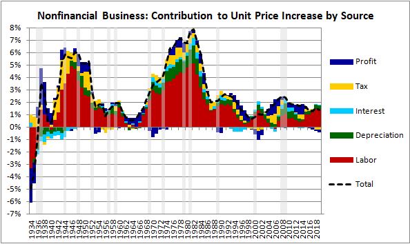
Focusing on the 1940's, we see that tax increases represented a significant component of the unit price increases that occurred during the period. These increases resulted from changes in tax policy—in particular, the introduction of the excess profits tax, discussed in the previous section. To be clear, the elevated representation of tax increases in the total doesn't necessarily mean that tax increases caused unit prices to go up. Instead, it means that tax increases took away inflation-related gains that would have otherwise gone to a different source—in this case, profit.
Focusing on the 1970's, we see that total unit price increases, represented as the dotted line in the chart, were not as high as actual end consumer price inflation (CPI). The reason is that the chart only includes components of unit price increases that were attributable to and that accrued to domestic entities. It excludes the component of price increases that were attributable to and that accrued to foreign entities--in particular, the foreign producers of imported oil. Increases in the cost of imported oil were significant contributors to the 1970's inflation.
Focusing on the recent period in the chart, we see that a significant share of the increase in unit prices that has occurred in recent decades has gone to shareholders in the form of higher profits per unit of production. Very recently, just before the pandemic hit, employees had been receiving a growing share of that gain, with labor costs per unit of production rising faster than other costs. The share of unit price increases going to lenders (via interest) and the government (via taxes) has been low and sometimes negative, reflecting the effects of falling interest rates and the Trump corporate tax cut, respectively.
Expansionary Fiscal Policy, Inflation, and Upside-Down Markets
Expansionary fiscal policy can provoke inflation through cost-push and structural mechanisms, but the core mechanism is demand-driven, grounded in demand-pull inflation. Demand-pull inflation is a state of excessive spending, so in assessing the inflationary risks of expansionary fiscal policy, we need to focus on the ways in which it can lead to excessive spending, not only in the present moment, but also in the future.
Over the long-term, expansionary fiscal policy increases spending by increasing the financial wealth of the private sector. We've used the term "wealth" repeatedly throughout the piece, but we haven't clearly defined it. Wealth is anything that has value. We can distinguish between two different senses of wealth: financial and real.
(1) Financial Wealth is wealth related to money, including promises to pay money and the capacity to sell things for money. Financial wealth is relevant to inflation because it confers spending power.
(2) Real Wealth is wealth related to the real goods and services that people want, including the capacity to produce those goods and services. Real wealth is relevant to inflation because it's the means by which spending power is fulfilled.
If we think of a given type of wealth—say, equity in a business with productive assets—the wealth is financial wealth in the sense that it yields cash flows and can be sold for money in a market. The wealth is real wealth in the sense that the underlying business produces real goods and services that people want to consume.
Whenever an entity—be it a person, a corporation, or a government—engages in productive deficit spending, that entity will increase the financial wealth, and therefore the spending power, of the overall system. To illustrate, suppose that I borrow money to start a restaurant business. I'm spending money in excess of my income and therefore I'm engaging in deficit spending. This spending will affect three parties in the system: the borrower (i.e., me, the restaurant investor), the lender, and the recipient of the money (i.e., the workers who build the restaurant). The financial wealth of each party will change as follows:
Borrower (no change): As the borrower, I take on a liability and use it to build an asset, a restaurant. Since the restaurant will generate future cash flows, we can conceptualize it as a financial asset. On this conceptualization, the deficit spending will not change my net financial wealth, since the new financial liability that I will have taken on will be offset by the new financial asset of equivalent value that I now own.
Lender (no change): The lender that issues me the loan will be trading cash for a financial asset of equal value—i.e., the loan that I owe him. His net financial wealth will remain similarly unchanged.
Recipient (increase): When I spend the money, the people that I spend it on—the architects, the construction workers, etc. —will receive it as income, without taking on any liabilities. Their net financial wealth will therefore rise.
The table below shows the financial wealth of the system before and after the event:
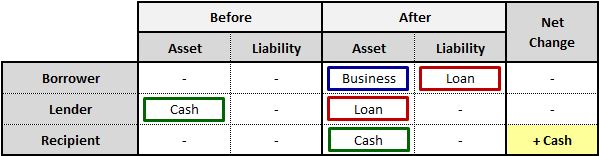
Tallying up the changes, we see that the total financial wealth in the system increases by the amount of cash spent in the deficit spending event. The borrower and the lender see no changes in their financial wealth, and the recipients receive the cash as a positive change. They now have additional spending power that they didn't previously have.
Now, over the long-term, the financial wealth in an economy needs to grow at a similar pace to the real wealth in the economy. If the financial wealth is allowed to grow faster than the real wealth, spending power will grow faster than the capacity to fulfill spending. The eventual result will be a condition of excess spending—i.e., demand-pull inflation.
For this reason, there needs to be a constraint on the process of deficit spending, a source of pressure that forces it to be deployed in ways that increase the economy's real wealth in proportion to the increases in financial wealth that are occurring. In a classical market-based economy, this constraint comes from the need to pay interest on liabilities and to eventually repay their principal in full. The constraint operates like an invisible hand—call it an "invisible fist"—that reins in and destroys financial wealth created through unproductive deficit spending, the liabilities of which cannot be properly financed or repaid.
In the example, the above constraint is satisfied because I invested the money in a productive asset, a restaurant. If the restaurant succeeds in delivering valuable goods and services that people want to spend money on, then the financial wealth in the system—i.e., its spending power—will have grown in proportion to the real wealth in the system—i.e., its capacity to fulfill spending. The appropriateness of the financial wealth increase will be reflected in the cash flows that the restaurant generates, which can be used to finance and repay the debt. All will be well.
But suppose that instead of using the borrowed money to build the restaurant, I waste it on a set of expensive vacations. My deficit spending will have created new financial wealth for the system, but it won't have created any new real wealth. The lack of real wealth creation in the expenditure will be reflected in the fact that there won't be any future cash flows coming my way to finance it, as there would have been if I had used the money to pay for the construction or acquisition of an asset that produced things that people wanted. So, what will happen? The answer: the invisible fist will rein in and destroy the financial wealth that was created, bringing the total financial wealth in the system back to where it was before the unproductive deficit spending occurred.
The first place where the invisible fist will destroy financial wealth will be on my personal balance sheet. I originally accounted for the business as a new financial asset that offset the new liability that I had taken on. If that new financial asset never comes into existence, or if it turns out to be worthless, then it's going to get written off. I'm going to end up with a new liability and nothing else—a negative cumulative hit to my net worth. If I had used the money to build the restaurant, I would have been able to repay the liability out of the cash flows that it would have gone on to generate. But since I wasted the money on vacations, I will have to repay the liability using other cash flows that I have coming to me. Ultimately, the need to divert those other cash flows will reduce my future spending power, compensating for the increased spending power that I wastefully conferred onto those who I bought the vacations from.
If my future cash flows aren't enough to repay the loan—and they probably won't be—then the next place where the invisible fist will destroy financial wealth will be on the lender's balance sheet. The loan will get defaulted on. In a full default, the lender will suffer a hit to his financial wealth equivalent in size to the financial wealth that I added to the balance sheets of the people that I bought the vacations from. The lender will experience an associated decrease in his spending power, compensating for the increase in spending power that my unproductive vacation expenditures will have conferred onto those people.
In the end, the total financial wealth and spending power in the system will be conserved. The invisible fist will not allow them to enjoy sustained increases, since the real wealth in the system—its capacity to fulfill spending—did not increase. In this way, the invisible fist will prevent an inflationary outcome in which the supply of financial wealth overwhelms the supply of real wealth. The process offers an excellent example of the natural elegance of a capitalist, market-based economic system, the elegance that Adam Smith famously marveled at.
The variable that determines the sensitivity and power that the invisible fist carries in an economy is the interest rate--specifically, the real interest rate, adjusted for price level changes that are occurring over time. When the real interest rate increases, the productivity stresses imposed on deficit spending increase. Borrowing to consume becomes more expensive in terms of the real amount that it subtracts from the borrower's future income. Deficit-financed investments are forced to overcome a higher hurdle. They have to be more productive, facilitating in the creation of goods and services that are more wanted by the economy, in order to attract the income needed to pay the higher interest expense. Imagine an extreme situation in which the real interest rate in an economy is set at 20%. The sensitivity and power of the invisible fist would be extraordinary. Borrowing to consume would lead to bankruptcy for almost anyone. Only those investments that facilitate in the production of desperately-wanted goods and services that can be sold with extreme pricing power would be capable of generating sufficient income to finance themselves.
The same concept applies in reverse when the real interest rate falls. The productivity stresses imposed on deficit spending get reduced. Imagine an extreme situation in which the real interest rate in an economy is set at -20%. Borrowing to fund consumption in the present moment and paying later with future income would be rewarded with a 20% annual gain relative to the alternative of saving in the present moment to fund the same consumption later. Likewise, deficit-financed investments would only need to be marginally profitable to be viable, facilitating in the production of goods and services that attract just enough demand to overcome the break-even point, since the real value of the debt would naturally dissolve away over time, falling by a half every three years.
The relationship between the invisible fist and the real interest rate translates into an important supply-side policy insight. In economic situations where there are many opportunities to add value to an economy through investment, and where those opportunities are crowding on each other, driving aggressive competition for a tight underlying resource pool, higher real interest rates will lead to better supply-side outcomes. They will strengthen the grip of the invisible fist, pushing out the less productive, less profitable opportunities that can't afford the higher rates and making room for the more productive, more profitable opportunities that can afford them. Conversely, in economic situations where opportunities to add value to an economy through investment are limited, and where significant portions of the underlying resource pool are sitting idle, lower real interest rates will lead to better supply-side outcomes, since they will weaken the threat of the invisible fist and help draw out any value-additive investment opportunities that are there.
The invisible fist's dependency on the real interest rate creates a potential path through which consumers and investors, as a group, can escape from it. By taking on large amounts of debt and unproductively spending the proceeds, they themselves, through their unproductive financial wealth creation, can generate an inflation that increases their nominal incomes and that reduces the real values of the debts that they've taken on. In a redeemable monetary system based on a real asset, e.g., gold, redemptions of the asset will prevent this outcome from occurring. In response to the inflation, economic participants will take their depreciating paper banknotes to the bank to get back the real asset—i.e., the gold—that underlies them. The redemptions will deplete the banking system's gold reserves, forcing it to curtail its lending and pull in existing loans in order to reduce the risk of defaulting on redemption requests. The reduction in lending and the attempt to call back outstanding loans will slow the inflation and drive an increase in interest rates that will bring the invisible fist back into play, typically in an uncontrolled, non-linear manner that leads to a smashing of the entire economy. In a modern fiat-based monetary system, the central bank will prevent the escape by hiking interest rates to stop the inflation. When the debts come due, they will come due at higher interest rates, revealing whose spending has been productive and profitable and whose spending has not been.
In addition to liability accumulation, another way in which the total financial wealth and spending power in an economy can increase is through asset price appreciation. To illustrate, suppose that I buy a penny stock and pump it to some absurd price. After the pump, I will be financially wealthier and capable of a greater amount of spending, given that I will own a marketable asset that can be sold for a larger amount of money. But this wealth will not be backed by any real wealth since the company produces nothing and generates no earnings. Over time, the invisible fist will find a way to destroy it. If the market is functioning properly, investors will come to realize that the company is worthless and will sell it down to fair value, deleting the gains in financial wealth and spending power that the pump brought about, gains that never should have occurred. If there's a broader asset bubble influencing the outcome, the bubble will deflate when the inflated level of financial wealth in the system creeps into consumer prices, driving a tightening of monetary policy that pulls the air out of the process.
All of the points that we've made so far about deficit spending apply with equal force to the government. When the government engages in deficit spending, it increases the financial wealth of the private sector, which receives the deficit spending as income without having to take on liabilities. Importantly, the gain in spending power associated with this increase is unaffected by the method through which the deficit spending is financed, whether through debt issuance or through direct money-printing. The associated assets—government bonds and cash—can be readily converted into each other in a market and are therefore functionally identical in terms of the spending power that they confer.
To illustrate with an example, suppose that the government uses deficit spending to pay unemployment insurance. The table below captures the balance sheet changes that the expenditure will bring about:
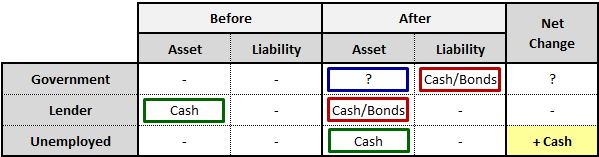
The unemployed person will not be affected by the method through which the deficit spending is financed—he will receive the same cash payment regardless. Instead, the entity that will be affected is the lender. If the government funds the deficit spending with debt, then the lender will end up holding a government bond in lieu of cash. If the government funds the deficit spending by printing money, then the lender will be entirely excluded from the process, and will continue holding whatever cash she was holding. The difference—holding bonds and holding cash—makes no difference to the lender's spending power, because the bonds and cash can be immediately exchanged for each other on demand in the market. If you have one, you effectively have the other.
Now, a currency-issuing government is unique in that it has the ability to bypass the constraints of the invisible fist. It sets the interest rate on the money that it borrows, and can ultimately print money directly, using the proceeds to make good on any liabilities that it owes. Since the invisible fist works through the pressures of having to pay interest on liabilities and eventually repay their principal in full, the government's ability to bypass these pressures prevents the invisible fist from destroying unproductive deficit-driven wealth. The government is the only entity with the power to destroy that wealth, a power that it can exercise by either running a surplus or by voluntarily choosing to default.
Because it can bypass the invisible fist, the government can set the total financial wealth of the private sector to be whatever value it wants, without worrying about how it's going to finance the liabilities that it has to take on in the process. This capacity is what makes it uniquely capable of arresting and reversing demand-driven downturns. If the private sector falls into a withholding trap, a situation in which everyone jeopardizes everyone else's income stream by withholding income, the government can immediately end the problem by injecting whatever amount of wealth and income it needs to inject in order to quench the withholding demand and stimulate desired levels of spending. In taking this action, it won't have to worry about financing the ensuing liabilities—in the worst case, it can finance them by simply printing up the necessary amount of money.
In response to this point, skeptics will rightly ask: how can a government create and inject new financial wealth—new potential claims on the economy's real output—without causing inflation, i.e., a depreciation in the value of existing claims? The answer lies in the fact that the vast majority of the potential claims that exist as financial wealth in the system are not going to be exercised in a given period, but will instead be held idle, as savings. Of course, some of the claims will be exercised, but as long as the economy has the capacity to fulfill those claims by delivering the wanted goods and services that people are seeking to purchase, then the rest of the claims can peacefully coexist together without depreciating each other.
If a sufficient number of claims in the system aren't going to be held idle as they need to be—if they're all going to be exercised at the same time in a spending frenzy—then the result can be inflationary at almost any level of existing wealth, even a fraction of the current level. For an illustration, consider the chart below, which shows the total net worth of all U.S. households separate, with the sum separated into different wealth percentiles, from 1952 through 2020 (source: FRED):
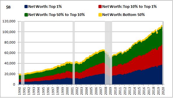
As you can see, the U.S. economy currently holds more than $100T of total net worth, a large portion of which could be spent tomorrow, if the owners wanted to spend it. Total GNP is roughly $21T, so even if only a fraction of this wealth were spent in a given year on top of what is already spent, the result would be wildly inflationary. But the point is, the vast majority of the wealth is not spent in a given year. The people holding it want to keep it and grow it—they don't want to lose it by spending it down.
Spending is a flow phenomenon, whereas wealth is a stock phenomenon. The addition of stock (wealth) to the private sector via government deficits can lead to an increase in flow (spending), but it doesn't have to lead to such an increase. If it does lead to such an increase, the spending will multiply by some factor, going from participant to participant as spending-turned-income-turned-spending, until it gets withheld. But if relevant participants in this chain are inclined to withhold the income rather than spend it, then the effective multiplier on the process can end up being small. The economy may have the spare capacity needed to fully accommodate the new spending, preventing an inflationary impact on prices.
Everyone wants to accumulate more wealth, but not everyone wants to accumulate it in order to spend it. Many people, especially those that already have sufficient amounts of it, want to accumulate it for psychological reasons—because they value the security, status, power, and sense of accomplishment that accumulating it brings. If the government prints new money and gives it to those people in exchange for valuable goods and services that can be transferred to others, the result can be a genuine "free lunch" for the system--the producers of the goods and services get the psychological benefits that wealth accumulation brings, and the recipients of the goods and services get to consume at no charge. Those holding existing financial wealth do not suffer any inflation in the process because the new wealth gets eagerly withheld, removed from circulation in a way that keeps aggregate spending below the economy's capacity to produce.
With these points acknowledged, we have to admit that the government's ability to deficit spend in a way that bypasses the invisible fist is a source of inflation risk. Without the invisible fist, there's nothing to stop the government from injecting more financial wealth into the economy than the economy can absorb in a non-inflationary manner. In lieu of the natural protection provided by market-based mechanisms, the onus is left on government officials to determine, without a reliable theory and without the ability to see the future impacts of their actions, how much future inflationary pressure they will introduce by injecting a given amount of unproductive financial wealth into the economy.
It's important to clarify that the inflation that we're referring to here is not the immediate inflation that can occur when a government directly spends money into an overheating economy or an overheating sector. That kind of inflation is about the government spending itself, which the overheated economy or sector can't currently support. If it's going to occur, it's going to occur regardless of how the spending is financed, whether through deficits, asset sales, taxes or whatever else.
Instead, the inflation that we're referring to is the longer-term inflation that can occur when the government makes the private sector wealthier on paper than it can afford to be in reality, in terms of its ability to produce the quantity and quality of goods and services that it will want at that level of wealth. With regard to that inflation, the deficit itself, which represents an unencumbered gift of wealth to the private sector, is the problem.
This point ties back to the concept of multiplication discussed in the previous section. When the government runs a deficit, it makes someone wealthier. The recipient may withhold the wealth, but she may also spend it, allowing it to multiply through the system as spending-turned-income-turned-spending. The critical variable that determines the extent of the multiplication that occurs in the process is the economy's withholding demand, the number of times the wealth has to get tossed around as income and spending before it falls into the hands of someone who wants to hold it rather than spend it. The capacity of an economy to absorb injected wealth in a non-inflationary manner is a function of that demand. Importantly, it's not a constant—it can change over time. If it does change, then a wealth injection that originally occurred without any sign of inflation could end up provoking inflation at a later time, possibly years later, when conditions supporting multiplier effects have improved.
To illustrate the point using the current pandemic as an example, one possible economic response to the pandemic would be to have the government use its fiscal power to replace 100% of any income losses that the pandemic causes. Under this approach, if a restaurant were to lose its customers and therefore its source of revenue, the government would create an amount of money equal to the lost revenue and give it to the business as a grant. Similarly, if a retail worker were to lose a job because a store closes, the government would create new money and use it to pay the worker's lost wages, with no expectation of eventual repayment. In a nightmare virus scenario, we can imagine a response of this type remaining in place for many years, forcing the government to incur a massive amount of fiscal debt—hundreds of percentage points worth of GNP.
In attempting to articulate the cost of such a response, we can't just focus on current inflation pressure—the inflation pressure that we see right now, at this precise moment. With the virus still swarming around inflicting damage, the private sector's elevated withholding demand and constrained ability to spend could easily be sufficient to prevent those pressures from taking root. What we have to focus on is the longer-term inflationary pressure that the injections will go on to introduce when the economy has returned to a normal state.
The fears and constraints that are currently keeping inflation down are not permanent fixtures of the economy. They're temporary consequences of the virus. In the future, when the problem of the virus is resolved, they will go away. But the previously injected wealth will not. It will remain in the system, free to multiply in an inflationary process. There are things that the government can do in the future to prevent the injected wealth from generating excessive inflation—for example, it can attempt to take the wealth back through tax increases and spending cuts, or it can attempt to increase withholding demand and discourage borrowing by raising interest rates. But these actions are politically difficult to implement and come with separate costs and limitations that need to be considered.
This concern isn't just theoretical. It actually played out in the aftermath of the only other large debt expansion that the U.S. government has ever taken on, the expansion associated with World War II. That expansion represented a massive injection of wealth into the private sector, the largest 4-year increase in private sector wealth in U.S. history21:
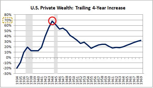
If the government's injection of financial wealth during World War II had been associated with investments that increased the economy's capacity to meet the kind of spending demand that an optimistic peacetime economy would be likely to exhibit, then it might not have become inflationary. Unfortunately, it wasn't associated with any such investment and couldn't have been, as it was needed to fund critical war expenditures. Unsurprisingly, as private sector withholding demand normalized in the aftermath of the war, and as war-related controls on consumption and credit expansion were lifted, the previously idle financial wealth began to freely circulate and multiply, generating a surge in overall spending that yielded significant inflationary pressure.
When an economy has too much financial wealth in it, evidenced by the inflationary pressure that it is experiencing, the available options, outside of onerous external controls (on prices, profits, wages, credit, and so on) are to either: (1) take the wealth out of the economy by running a government surplus, or (2) incentivize the withholding of the wealth and discourage the borrowing of it by raising interest rates.
For the first option, the politically attractive strategy of generating a surplus by taxing billionaires probably won't be sufficient. Billionaires have an extremely low propensity to spend marginal income and wealth, and therefore reductions in their income and wealth do not meaningfully affect overall spending. Instead, the government will likely have to achieve the surplus in ways that reduce wealth and income more broadly. Few politicians want to be responsible for policies that have this effect, which is why government surpluses aren't particularly reliable options for managing debt-driven inflations.
The more feasible option is the second option, raising interest rates. The risk-free interest rate is the compensation that economic agents receive in exchange for withholding money, and also the cost that they pay to borrow and spend it, before considering risk. By increasing that rate, central banks increase the economy's propensity to withhold and weaken its propensity to deficit spend, reducing inflationary pressure.
But there's an important caveat. Interest is itself a form of income. If the stock of government debt in the economy is extremely large, then raising interest rates can have the counterproductive effect of increasing overall private sector income, which can in theory make inflation worse, not better. The relationship between the amount of debt in the system and the overall amount of interest income that has to be paid to it has the potential to become non-linear. More debt means more wealth in the system, which means a greater need to get people to withhold, which means a higher interest rate needed as an incentive. Paying a higher interest rate on each unit of a larger sum of debt is multiplicative through two channels, not one, hence the non-linearity.
To illustrate the non-linearity with a concrete example, at the pre-pandemic U.S. federal government debt level of around $20T, you might have only needed to pay 1% to the owners—$200B per year—at the cycle peak to achieve the levels of withholding sufficient to keep inflation on target. If you were to increase the debt amount by 10X, to $200T, you would almost surely need to pay an amount more than just 1% to keep it sufficiently withheld—you'd probably have to pay something closer to 5%, if not higher than that. The total interest income that you would have to pay out would then rise from $200B to $10T, an increase of 50x relative to a debt increase of only 10x. Paying $10T, 50% of GNP, in annual interest income would itself be highly inflationary and would further increase the interest rate that you would have to pay to keep the wealth withheld, creating a potential spiral.
Notice that we've ignored the question of whether the government can "afford" the interest expense on the debt. That question is not properly framed, since a government that prints its own currency can afford to pay any nominal quantity, no matter how large. The right question to ask is not whether the government can afford the interest expense (it can), but whether the real economy can support the increased spending that would result from paying that expense out as income to holders of cash and government bonds.
In the case of World War II, political considerations prevented the Federal Reserve from appropriately responding to the inflation pressure that emerged in the aftermath of the war. At the insistence of the Treasury, the Fed kept rates near zero and allowed the inflation pressure to proceed unchecked. As a consequence, inflation accelerated into the double digits, and anyone who was unfortunate enough to be holding money in a savings bond or in a bank went on to suffer a dramatic loss of real wealth—more than 25% over the three-year period that followed the war—without receiving any remuneration in the form of interest (source: FRED). This loss was very different from the temporary mark-to-market losses that equity investors experience when sentiment fluctuates. It was a permanent loss of capital, fully unrecoverable, inflicted on bondholders and bank depositors that were never exposed to the prospect of gains.
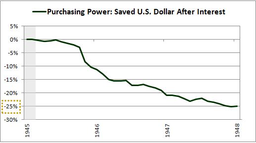
In weighing the risk of a similar inflationary outcome in the case of the COVID-19 fiscal expansion, some will ask: Why do we have to view such an outcome as a bad thing? Why can't we just accept it as the necessary cost of government spending? Economists can come up with economic reasons why the derivative effects of an inflation of this kind might hinder economic growth, but those reasons would fail to capture the true concern. The true concern is grounded in fairness. Inflation destroys the wealth of people who are holding their savings in the form of money and debt. To earn whatever financial surplus they are currently holding, those people did work and added value to the system. Inflation prevents them from getting that value back. It effectively confiscates the value and arbitrarily redistributes it to those who are holding real assets, to include real labor assets.
Principles of fairness would suggest that if earned wealth is going to be permanently taken from people in order to fund important government spending, it should be taken broadly from everyone, based on progressive considerations such as how much wealth a person already has. But inflationary fiscal policies don't operate in this way. Instead, they target people who lack the financial cleverness to foresee the inflation and shelter their wealth from it. Those people end up paying the entirety of a bill that is owed by everyone.
To the unfortunate people who lost large chunks of their wealth in the post-World-War-II inflation, we can certainly put the blame back on them—"It was your fault for being stupid, you should have foreseen the inflation and sheltered your wealth from it in stocks or in real estate." But someone had to hold the paper assets that the government created to fund the war, and therefore someone had to be the eventual bag-holder in the inflationary outcome that ensued. If it hadn't been them, it would have been whoever they bought stocks and real estate from. Their decision to hold the assets may have been stupid in hindsight, but the point is, it's wrong to single out the stupid and have them pay for government spending. We all should pay for that spending, based not on our investing guile, but on our ability to pay.
These observations lead us to the trillion-dollar question: if the COVID-19 stimulus were to become inflationary in the same way that the deficit spending associated with World War II was inflationary, how might U.S. policy authorities—specifically, Congress and the Fed—respond? And how would financial markets react?
The odds that Congress would be able to identify and come to agreement on the right kind of spending cut or tax increase to address the inflation—for example, a cut in government benefits or a tax increase on consumption, both of which would hit regular people in a noticeable way—is almost zero. The most likely response would come from the Fed, which has a 2% inflation target.
If the Fed's response would be to abandon its inflation target and let the inflation run—as it did in the aftermath of World War II—then stocks would have a field day. Long-term bonds might sell off a bit, but if the Fed signaled its intention to hold short rates at low levels in the presence of the inflation, the selloff would be slowed by the arbitrage opportunity that would emerge in conjunction with the rising term premium. If the Fed committed to actively holding down long-term interest rates through yield curve control, as happened during and after World War II, then then there wouldn't be any selloff at all.
Historically, inflation has been associated with lower equity valuations. Some have used this fact to argue that an inflationary outcome to COVID-19 would imply a negative outcome for equities, regardless of how the Fed chose to respond. But the association between inflation and reduced valuations is not a consequence of any inherent aversion that stocks have to inflation. Much of it is instead due to a single coincidence: inflation has tended to occur during and after wars, and wars are risk-off events that drive contractions in equity valuations. The remainder of the association is likely due to accounting factors and policy feedbacks:
(1) Overstated Earnings: Inflation leads to understated depreciation in GAAP and therefore overstated earnings. Overstated earnings warrant lower P/E multiples.
(2) Policy Response: Inflation leads to interest rate hikes, which (a) make stocks less attractive relative to cash and (re-priced) bonds and (b) increase corporate interest expense as well as the risk of financial instability, bankruptcy, and recession.
If the Fed were to take away (2) by affirming its intention to hold rates at low levels despite elevated inflation, then stocks wouldn't have any reason to become cheaper relative to properly-measured earnings. In fact, they would have good reason to become more expensive, given that they are one of the few asset classes that can protect investors from the wealth losses associated with inflation. If you disagree with this point, then have a look at a chart of local currency stock performance in Venezuela (IBC) or Iran (TEDPIX) during their recent respective inflations. You will quickly be convinced (source: TSE):
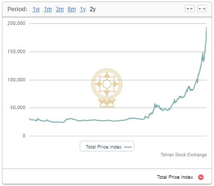
Now, if the Fed's response would be to address the inflation, raising rates as needed to keep it on or near the 2% target, then markets would turn upside-down. Things that investors normally consider to be good news, like rising consumer spending and falling unemployment, would turn into bad news, given their implications for future policy. The effect would be even stronger in the current market, given the extent to which low interest rates have fueled historic increases in equity valuations. If we found out tomorrow that the economy was going to need a sustained 6% long-term nominal rate to continue to inflate at the 2% target, much of that appreciation would be given back, with losses that could exceed the losses experienced during the worst part of the COVID-19 decline. The ensuing financial market damage would likely be deflationary, lowering the interest rate needed to keep inflation on target and assisting in the stabilization of markets--another reflection of the upside-down feedbacks that policy can introduce.
We can efficiently describe the upside-down dynamics that fiscal policy can introduce in an inflation-targeting monetary policy regime through the concept of the natural rate of interest, r*. I want to define r* slightly differently from usual, as the real, inflation-adjusted interest rate necessary to achieve stable inflation at a specific target value. If an economy would need a nominal interest rate of 0% to achieve stable 2% inflation, then its r* would be -2% (=0%-2%). If it would need a 2% rate, then its r* would be 0% (=2%-2%). If it would need a 4% rate, then its r* would be 2% (=4%-2%). And so on.
Over the long-term, inflation-targeting central banks are going to set real short-term interest rates somewhere near r*, and therefore the real rate of return on the risk-free fixed income assets that compete with equities will tend to converge on that rate. Right now, under current economic conditions, the rate is believed to be solidly negative, which is why risk-free fixed income assets are priced for negative real returns across the curve. The unattractiveness of these returns is one of the main reasons, if not the main reason, why equities currently trade at historically expensive valuations.
If the wealth that the government injects through the COVID-19 deficits eventually finds its way onto the balance sheets of wealthy individuals with a low marginal propensity to spend, then it will be withheld and will not have an appreciable effect on r*. But if the wealth instead circulates continually in the real economy, with sustained multiplicative impacts on income, spending, investment, and so on, then it will push up on r*. Assuming that the central bank remains responsive, real interest rates on the fixed income instruments that compete with equities will then rise, putting downward pressure on equity valuations in an upside-down outcome.
For an extreme illustration of the point, suppose that over the next few years, the U.S. government were to print up and give out a truly massive amount of new money—say $100T, roughly 500% of GNP, $300K per person. If you don't think that this number would be sufficient to induce strong inflationary pressures, then use whatever number you think would be sufficient—$250T, $500T, $1Q, etc.
For inflation to remain at 2% in the presence of such a large wealth injection, the wealth would have to be withheld at a very low multiplier. Even the slightest circulation of the wealth in the form of consumption and investment spending would strain the economy's productive resources and fuel an inflationary outcome. The interest rate incentive, r*, that would be needed to keep the injected wealth withheld at a low multiplier would therefore be very high—10%, 15%, 20%, maybe higher.22
If the Fed were to remain committed to keeping inflation on target in such a scenario, including by raising interest rates to extreme levels as needed, then one of two outcomes would ensue. Either:
(1) Runaway Inflation: People would want to spend the money and would spend it regardless of how much interest compensation they were offered in exchange for withholding it. The massive amount of interest income that would have to be paid out to incentivize people to withhold the money—worth 50% of GNP at a 10% rate (=500% X 10%)—would drive additional spending, counteracting the intended effect of the higher interest rate. The result would be runaway increases in spending and inflation that monetary policy would not be able to control. These increases would be accelerated by fears of inflation, introducing the risk of hyperinflation--a panic-driven run on the currency itself. The only available options to contain the process would be: (a) extreme levels of taxation—ideally wealth taxation, which would allow the government to rapidly take the wealth back and (b) price, profit, wage and credit controls across the economy, including controls on financial markets.
(2) Equity Market Adjustment: The Fed's interest rate increases would succeed in generating the necessary amount of withholding, bringing the inflation under control. Equity markets would then find themselves under pressure on multiple fronts: first, from overvaluation relative to cash and bonds, which would be offering significantly higher yields; second, from the increased interest expense that corporations would have to bear; third, from the increased unit labor costs associated with the elevated demand condition in the economy; and fourth, from the need to raise taxes, possibly corporate taxes, to help finance the compounding government interest burden.23 If the Fed were successful in limiting unit price increases to its 2% target, then the only revenue growth that corporations would be able to generate to offset these factors would be the real revenue growth that they generate by increasing their productive output. This source of growth would be nowhere near enough to offset the effects of rising costs and increased competition from high-yielding cash and bond alternatives. From a fundamental perspective, we would therefore expect to see equity prices decline.24
Outcome (2) would represent a classic upside-down outcome. The government hyper-stimulates the economy by giving households large amounts of money, and the gift ends up forcing a monetary policy response that outweighs the original effects of the stimulus itself, bringing about a decline in equities rather than an increase.
Returning to the COVID-19 wealth injection, our commentary so far has identified different paths that the Fed might take in responding to potential future inflation pressure, but it didn't actually specify which path the Fed is most likely to take. The Fed has been very clear that it's going to maintain a dovish bias, with a preference for keeping interest rates near zero, until inflation proves itself by exceeding the 2% target. The question is whether inflation will actually prove itself in that way. When the virus is resolved and a future administration is doing whatever it is doing on the fiscal front, what will r* actually be? And if rates are kept below r* in a slow, hesitant monetary policy response, what will happen to prices—not only the prices of consumer goods and services, but also the prices of important asset classes such as housing? If nothing will happen, if the inflation trend will stay roughly where it is, somewhere slightly above 2%, then the policy bias is likely to remain dovish, with rate increases occurring more slowly and with more caution than they would have in the past. But if the inflation will continue to creep higher, then policy biases will shift, and we will see a more deliberate response. Given the Fed's recent experience of having gone too far in raising rates, the Fed will continue to exhibit a bias against "too much tightening." But the felt sense of what constitutes "too much tightening" will change.
Right now, an inflation-fighting monetary policy mindset is not needed and hasn't been needed for a very long time. If the fiscal expansion that we've seen eventually causes such a mindset to become needed, the process of getting into that mindset, and of developing the confidence to act on it, will take time. Nonetheless, I think it's important to consider a few counterpoints when evaluating the massively dovish expectations that market participants currently have around the Fed's future path: (1) Deeply negative real interest rates are not a comfortable settling place for an economy. If a supportive fiscal backdrop makes it possible for inflation to satisfy the Fed's targets under real interest rates that are less negative and closer to zero, the Fed will feel at least some pull to move in that direction, and (2) When outcomes are moving away from targets, policymakers prefer action over inaction, even if the action is small. If fiscal policy ends up providing the fuel needed for inflation to overshoot the Fed's targets, it will be harder for the Fed to sit on its hands and leave rates at zero than people currently think, especially if asset markets are running wild (which, absent a Fed response, they probably will be) and if the cause of the original weakness--the virus--is gone.
The Fed's Monetary Response to COVID-19: Assessing the Inflationary Potential
In response to the COVID-19 pandemic, the Fed has stepped in and monetized the government's entire fiscal issuance, adding more than $3T to its balance sheet. Will this monetization prove to be inflationary?
To properly answer the question, we need to revisit a few earlier points made in passing. Inflation is a condition of too much spending, which can result from too much spending power. With respect to spending power, the form of government debt—whether investors hold it as government bonds or as cash monetized through central bank asset purchases—is irrelevant. Government bonds and cash are readily exchangeable for each other in markets, so if you have one, you effectively have the other. There is no realistic scenario where receiving a newly-issued government bond as payment in lieu of cash will prevent you from spending the present market value contained in the bond. If you wanted to spend that value, you could easily sell the bond for cash and spend it.
To be fair, it's conceivable that the money supply in an economy could get so tight that selling a bond near its fair market value becomes impossible. Imagine, for example, a hypothetical situation in which the Fed creates its own debt securities and sells them in an amount sufficient to shrink the money supply down to almost nothing—say, $1,000 across the entire U.S. economy. The required velocity that the $1,000 would need to travel at in order to satisfy the economy's demand to transact in existing wealth would be prohibitive, freezing up the market and undermining the exchangeability described above. But the Fed is not currently shrinking the money supply in this way. In fact, it's doing the opposite—it's expanding the money supply through asset purchases. Importantly, the fact that shrinking the money supply through asset sales can impair transactions and depress prices doesn't mean that increasing the money supply through asset purchases will fuel transactions and inflate prices. Liquidity is a condition for transactions and for price support, it's not their cause. Once a system is saturated with it, the impact of adding more of it rapidly drops off to zero.
Central bank purchases of long-term government bonds increase the prices of those bonds through two mechanisms—first and most obviously, through the direct addition of attempted buying flow into the bonds, and second, through the shrinking of outstanding supply in the bonds, which occurs alongside an increase in the supply of cash. Increases in the prices of the bonds can lead to increases in the prices of other asset classes, yielding general increases in the mark-to-market value of the overall asset universe. In this limited respect, central bank purchases can add wealth and spending power to the private sector. But the addition is not normally inflationary, because it only affects those with significant asset holdings—a small portion of the population with an extremely low propensity to spend marginal asset-related gains.
In using asset purchases to drive down the yields of long-term government bonds, and of all long-term bonds by substitution, central banks can reduce the incentive that investors have to commit to withholding wealth over the long-term, and also increase the incentive that borrowers have to commit to borrowing it over that term. This effect can stimulate consumption and investment spending from both sides, but it's not any different in principle from the effects that central banks exert when they control interest rates at shorter maturities. When central banks lower the interest rate on cash, they reduce the incentive to withhold wealth over the short-term and increase the incentive to borrow and spend it over that term. Importantly, the purpose of adjusting interest rates in this way is not to "help" or "hinder" the government in its efforts to fund itself, but rather to manage the level of spending that the economy will experience given the amount of wealth and spending power contained inside it, so that inflation can be maintained on target.
In the aftermath of the pandemic, we've seen the broad money supply (M2) explode. Many investors have expressed shock at the increase, expecting it to yield inflation (source: FRED):
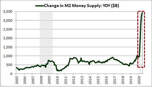
But the increase is primarily an artifact of the Fed's asset purchases, which the Fed has been conducting at an extraordinarily rapid pace. When the Fed purchases treasury bonds, agency bonds and other fixed income assets from private investors through bank dealer intermediaries, it takes those assets, which don't count as part of the broad money supply, and converts them into cash, which does count as part of the broad money supply. The broad money supply therefore increases. The increase isn't inflationary, however, because it doesn't entail an actual increase in the wealth and spending power of the private sector. All it represents is a change in the form of that wealth and spending power, from prime, marketable fixed income assets into almost the same thing: money.
Now, the point that I just made, that the Fed's asset purchases increase the broad money supply, is 100% analytically certain—there can be no doubt whatsoever as to whether it's true. Just think, if the Fed's purchases didn't increase the broad money supply, then the private investors that ultimately sell their bonds to the Fed would not be receiving money in exchange for the assets that they're selling. If they aren't receiving money, what are they receiving? Does the Fed steal the bonds from them? Or does it pay them, using new money that it creates?
Despite being analytically certain, this point can be difficult to empirically prove because "broad money" can take different forms inside the banking system. As a definition of "broad money", M2 arbitrarily includes certain categories of banking system money, such as normal checkable deposits, but excludes other important categories, such as large time deposits. Movement of money across these categories over time can hide the impact that the Fed's asset purchases have on the money supply. Fortunately, we can uncover the hidden impact by including all liabilities of the banking system in our definition of money, not just the specific types of deposit liabilities that M2 has been defined to include.
The chart below shows raw year-over-year (YOY) changes in the aggregate balance sheet—assets and liabilities—of U.S. banks from January 1974 through June 2020 (source: Fed H.8):
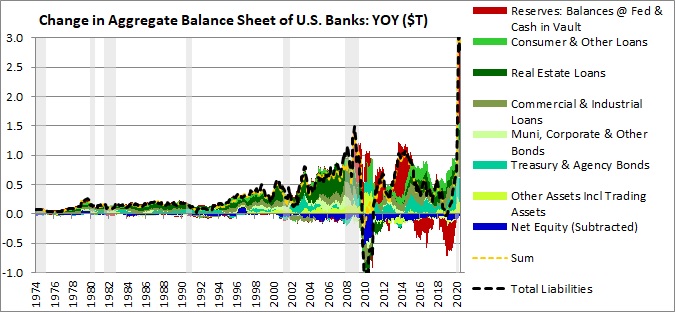
Let's briefly explore the major categories in the chart:
Bank "credit" assets, which include all bank loans and all bank securities holdings, are depicted in varying shades of green. When banks create these assets—for example, by lending to homeowners or by purchasing the bonds of municipalities—they create new deposits (liabilities). These new deposits literally are the "money" being lent out or used to fund the purchases. Their creation leads to an increase in the broad money supply as we've defined it, a point holds true regardless of whether the new deposits end up in the form of checkable deposits, small time deposits, large time deposits, or whatever else. All of these categorizations constitute liabilities of the banking system and therefore they all count as broad money under the definition that we're using.
Bank "reserve" assets, which include the balances that banks hold on deposit at the Fed and the paper bills and metal coins that they hold in their vaults, are shown in red. These assets represent the banking system's cash liquidity. Where does this cash liquidity come from? It comes from Fed asset purchases. When the Fed buys assets from private investors, the money that the investors receive ends up inside the banking system, represented as deposits (of those investors) on the liability side of bank balance sheets and as cash reserves on the asset side. Notably, the proceeds end up as cash reserves regardless of what banks choose to do with the reserves. Any movement of the reserves, through lending or spending or whatever else, will simply constitute a movement of the reserves from one bank to another. Unless depositors take the reserves out of the banking system by literally cashing paper bills and metal coins out of their accounts, some bank in the system will end up holding them, at all times.
To reiterate this critical point, banks can't do anything to change the aggregate supply of reserve assets in the system. Any movement of reserves—as occurs, for example, when you cash a check issued by one bank at another bank—will simply be a movement from one bank to the other. The only entity with control over their supply is the Fed, which has the power to change government bonds and other assets into cash through open market operations.
Bank "equity", which is the difference between bank assets and liabilities, is shown in blue. The sum of all bank assets, with bank equity subtracted, is shown as the dotted yellow line. The total liabilities of the banking system—which we've adjusted to exclude domestic interbank liabilities—is shown as the dotted black line. The dotted yellow line tracks almost perfectly with the dotted black line, confirming the chart's accuracy, given that that total assets minus equity equals total liabilities.
The chart below zooms in on the "pre-QE" period from January 1974 through December 2006. During this period, almost all growth in the money supply arose out of credit expansion—i.e., lending—with the Fed's open market operations making small contributions that were entirely negligible:
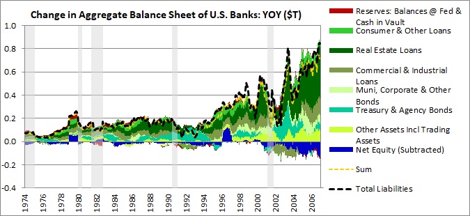
As you can see, almost all of the growth in liabilities mapped on to growth in bank credit assets, shown in various shades of green. These assets included: consumer loans, real estate loans, commercial and industrial loans, municipal, corporate, and other bond purchases, treasury and agency bond purchases, and purchases of other types of assets for trading, including equities. Growth in net reserves, which is what Fed asset purchases create, represented a negligible share of total growth.
The chart below zooms in on the "post-QE" period from January 2007 through June 2020. This period differs from the previous period in that quantitative easing (QE)—the central bank's use of asset purchases as a form of stimulus—became a recurring feature of monetary policy, with noticeable impacts on the quantity of liabilities in the banking system and on the broad money supply as we've defined it:
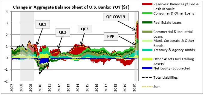
You can see the impacts of the Fed's QE1, QE2, and QE3 programs in the chart. Each of these programs led to a significant increase in the quantity of reserves held by the banking system. These reserves represented the asset side of deposit liabilities to private investors, and therefore their increases were associated with increases in the broad money supply, i.e., the total dollar amount of liabilities owed by the banking system. But the increases didn't always perfectly correlate with the overall growth in the money supply, since other contributors to that supply sometimes contracted in a way that happened to offset them. For example, during QE1, in the aftermath of Lehman's failure, commercial and industrial loan growth went negative, as did growth in loans to consumers, making the positive impact of the asset purchases on the money supply harder to detect.
If you look closely at the right side of the chart, you will see the huge jump in total bank liabilities that has recently occurred. That jump is essentially the same jump seen in the earlier chart of M2. The primary driver of the jump is the Fed's aggressive COVID-19 asset purchase response (QE-COV19), which has caused the sharp reserve increase shown in red. Another important contributor to the growth is the paycheck protection program (PPP). Loans from that program are accounted for in H.8 as "commercial and industrial loans." They reflect the government's efforts to shore up strained liquidity conditions in the corporate sector and prevent unnecessary layoffs and bankruptcies. The loans do not reflect strength in consumption or investment demand and are therefore unlikely to facilitate inflationary pressure. The government has had to step in and insure them because the private banking system, despite being in good financial shape, is neither willing nor able to take on the COVID-19 risk of the entire U.S. corporate sector all at once.
Now, some readers might be concerned with our inclusion of all bank liabilities in the definition of broad money. The definition reluctantly includes liabilities such as bonds and commercial paper that normally would not be included. In theory, we could try to take those liabilities out, but the problem is that the banking system is all one big pot. If we try to pull certain liabilities out of the pot, we're going to have to pull out certain assets—which assets are we going to pull out? Any choice of a category from which to pull will be arbitrary and will inevitably distort the results of the analysis. So instead of going down that path, we've simply defined "money" to include all of the banking system's liabilities, showing empirically that QE directly increases them.
In defense of this approach, the chart below shows the growth in bank liabilities by type from January 2007 to present:
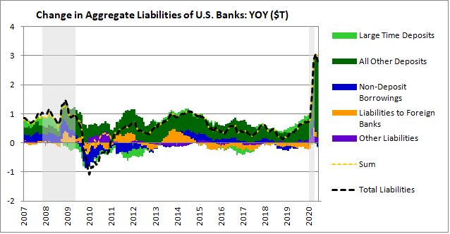
As you can see, the primary contributor to overall liability growth has been growth in deposits, shown in varying shades of green. Non-deposit borrowings—e.g., bond and commercial paper issuance—represent a small and bidirectional contributor to the total.
The chart helps to illustrate the ways in which the form of bank liabilities can change over time, with the owed money moving across different liability categories. If the money supply is arbitrarily defined to include certain types of these categories and exclude others, then movements across the categories will create the illusory appearance of money creation or destruction. These movements are not relevant to inflation, and therefore it doesn't make sense to define money in ways that are sensitive to them.
Returning to the alleged inflationary impact of the Fed's COVID-19 asset purchases, if the treasury bonds, agency bonds and other bonds that the Fed is currently buying were offering attractive yields, then the Fed's act of driving them down to unattractive levels through asset purchases could conceivably reduce investor withholding demand and make investors more likely to invest the underlying wealth. Similarly, if current long-term borrowing rates imposed significant costs on households, then the Fed's act of lowering them through asset purchases could stimulate borrowing, encouraging consumers to go out and buy cars, homes, and so on.
But in the current environment, the yields on safe fixed income assets are already very low and the cost of borrowing for prime borrowers is already very cheap. The effect of lowering those yields and costs further—say, from 1.5% on the 10-year treasury to 0.6%, or from 3.5% on the 30-year mortgage to 2.9%, is not likely to change behaviors in a significant way. If you preferred to hold wealth in a bond at 1.5% when you could have invested in the real economy, then you will probably prefer to hold wealth in a bond at 0.6% or cash at 0% over the same option—the difference is barely equal to a management fee. If you've found a home you want to buy, it's hard to envision a scenario where the difference between a 3.5% mortgage rate and a 2.9% mortgage would change your mind. For these reasons, we should be skeptical of the potential for the Fed's asset purchases to generate inflation.
Another proposed pathway through which the Fed's asset purchases might produce inflation is through the banking system. As explained above, asset purchases replace bonds in investor portfolios with cash that ultimately gets deposited in the banking system and held in reserve. If the supply of reserves in the banking system directly affected the ability of banks to lend, then the purchases might be able to contribute to an inflation by increasing bank lending. But in reality, under the current banking system setup, there's no relationship between reserve supply and bank lending capacity, and therefore there's no reason to expect any effect.
The required reserve ratio is currently set at zero, which means that from a regulatory perspective, banks don't need to keep any reserves on hand in order to lend. Even before the ratio was lowered to zero, the system was already heavily oversaturated with reserves. Banks were able to take advantage of any attractive lending opportunities that came their way while maintaining their reserve levels well above institutionally-preferred minimum levels and regulatorily-imposed minimum limits. If they needed to increase their reserves to stay above those minimum levels and limits, they were able to use the Fed Funds system to borrow reserves at the overnight rate, which they can still do. Under the current banking system setup, the considerations that impact their ability and propensity to lend have nothing to do with reserves and everything to do with: (1) the short-term interest rate, i.e., the interest rate paid on excess reserves (IOER), which is the cost of borrowing reserves for regulatory purposes and also the opportunity cost of lending in general, and (2) the margin to regulatory capital ratio limits, which banks cannot increase through borrowing and which Fed asset purchases do not affect.
Thinking through the impacts, then, there's no reason to expect the Fed's asset purchases to appreciably contribute to an inflation in the current environment. Fed critics, of course, will respond by arguing that the purchases contribute to a different type of inflation—asset inflation. As evidence, they will point to the powerful stock market rally that has occurred every time the Fed has initiated asset purchases, including under "not QE" auspices.
There's no doubt that central bank purchases can push up on asset prices, acting through portfolio preference channels as well as through placebo effects. But with respect to the COVID-19 stock market rally, it's not clear that the Fed's purchases have been a significant contributor to the price increases that have occurred. Some of the rally is surely attributable to the Fed's efforts to re-liquify and backstop the corporate bond market, but the real driver of the rally has been the unexpectedly strong fiscal response, which has dramatically boosted corporate revenue, profit and solvency relative to what they would have otherwise fallen to.
For evidence, consider the market's reaction to each Fed announcement in the run-up to the eventual market bottom. The Fed announced its first rate cut on March 3rd, 2020. The market blew off the news and kept falling. On March 15th, the Fed cut rates to zero and initiated the most aggressively-paced quantitative easing program in economic history. Once again, the market blew off the news and continued to make new lows. For the duration of the ensuing week, the Fed continued to announce new purchase programs and facilities; the market continued to fall. On the morning of March 23rd, the Fed announced a program to backstop the corporate bond market, crossing a rubicon that many believed would never be crossed. The market initially rallied, but then gave back all of its gains, closing the day near the lows. When did the sustained market rally finally begin? On the evening of March 23rd, when it became clear that Congress was set to pass the biggest fiscal spending package in the country's history, a package that was several times larger than initially expected.
The U.S. Government's Fiscal Response to COVID-19: Assessing the Inflationary Potential
The COVID-19 pandemic represents a situation in which there's an urgent need to provide high levels of financial support to households and corporations. Most people would agree that this support should be provided. The question is, over the long-term, how should it be funded? What portion of the funding should come from government debt accumulation, and what portion should come from increases in taxation or reductions in spending in other areas? To answer this question, we need to understand and quantify the true constraints that we face in the amount of government debt that we can afford to take on.
Importantly, these constraints are not financing constraints on the government. A sovereign government has the capacity to pay interest and principal on any amount of debt that it takes on in its own currency, right up to infinity. Instead, the constraints are constraints on the amount of financial wealth that the private sector is willing to passively absorb in that currency. Government debt accumulation injects financial wealth into the private sector, and financial wealth is spending power. How much spending power can the government inject into the private sector before it pushes actual spending above the level that the economy's productive capacity can support? More specifically, how much spending power can it inject before it creates conditions under which harmful policy responses, to include those highlighted below, become necessary to keep inflation on target?
Interest Rates: Large increases in real interest rates that strain indebted portions of the private sector, that disincentivize necessary productive investments, and that necessitate tax increases to fund elevated government interest burdens.
Taxes: Large increases in income taxes that discourage production and that shift valuable resources into useless tax avoidance. Large increases in wealth taxes that drive capital flight. Large increases in consumption taxes that further inflate final prices.
Controls: Price, wage, profit, and credit controls that infringe on economic liberties and that suppress necessary supply-side responses.
The answers to these questions define the true fiscal limits that are in effect.
In thinking about the limits of fiscal policy, we should not be lulled into complacency by the U.S. economy's recent lack of inflation. There is a limit, a point at which fiscal expansion would trigger an inflation that would only be controllable through the use of unacceptable interventions. We may not know where that limit is—whether it will come in to play at a Debt-to-GDP ratio of 150%, 200%, 250%, 500%, 1,000%, 2,000%, 100,000%, and so on. But we can be sure that it exists somewhere, right now, as we embark on an effort to explore it.
The process of identifying optimal macroeconomic policies is a complex process unto itself. We can aptly describe it with a sports analogy. In every sport, players evolve over time to become more sophisticated, using unorthodox techniques to gain an edge. In tennis, for example, players start out by learning simple racket grips and natural striking techniques—move your arm, hit the ball. But as they progress into professionals, they learn to put on weird grips and to strike the ball at oblong angles, achieving violent spins that help them win.
Over time, the same type of evolution takes place in the arenas of monetary and fiscal policy. Policymakers learn how to optimize economic outcomes by going beyond the "basics" and applying their policy tools in unorthodox ways. In the aftermath of the two most recent crises—the Great Recession and COVID-19—this learning process has been occurring at an accelerated pace. Many of the lessons being learned, of course, were learned a long time ago. They were forgotten, and are now being re-learned.
In the arena of fiscal policy, the "traditional" approach to identifying fiscal constraints is to assume that governments are like households and corporations, subject to the same pressures of the invisible fist. On this approach, we assume that any debt that the government takes on will have to be financed, and that the government won't be able to finance it by cheating the process, i.e., lowering the interest cost of the debt down to negligible levels or obtaining funds by "printing money." Operating on this assumption is useful because it helps ensure that the money that the government borrows gets invested in a productive manner. If the borrowed money doesn't get productively invested, if it gets consumed away, then its cost will have to be paid out of the government's existing resource base. The government will have to increase taxes and cut spending, which will pull the financial wealth injected by the debt accumulation back out from the system, preventing it from fueling an inflation. If the will or capacity to implement these changes isn't present, then the injected wealth will get removed through a more violent mechanism—government default. By conceptualizing the government as if it were constrained in this way, unable to lean on a captured central bank or a printing press, we allow the invisible fist to enforce proper discipline on it, preventing inflationary outcomes.
We will eventually learn, of course, that the pressures of the invisible fist are artificial. If we want to, we can use the power of money creation to bypass them—not only in the funding of the government's deficit spending, but in the funding of the deficit spending of anyone that we, as a society, want to help. When we realize that we can bypass them, we enter the "top spin" realm of tennis sophistication described above. We gain access to a tool that can optimize economic outcomes and avert human tragedies. Because it's an extremely powerful tool, it's a tool that can also cause harm.
If we're going to bypass the artificial constraints of the invisible fist--and we often should—we need a way to quantify the true constraints that we face. How much financial wealth can we inject into the economy before we provoke unacceptable outcomes? That amount is our true fiscal constraint. In an ideal world, the optimal way to quantify it would be through experiment. We would use deficit spending to actually inject a desired amount of financial wealth into the economy—say, $1T—and then wait to see what happens over the medium and long-term. In the case of the COVID-19 pandemic, we would wait for the underlying problem--the virus--to get resolved and for the world to return to a normal state. We would then ask:
How much inflationary pressure emerges?
How high do we have to raise future interest rates and tax rates to keep the inflationary pressure in check?
Can we accept those increases, or would we have to instead shift the losses onto unwitting bondholders and bank depositors?
We would gather the answer to these questions from actual empirical observations of the economy, and then rewind the universe back to where it was and re-run the experiment, increasing the amount of wealth injected each time. After trying $1T, we would try $2T, then $3T, then $4T, ..., then $98T, then $99T, then $100T, and so on. Continuing in this way, we would eventually reach a point where we would not be able to keep inflation on target using policy actions that we consider to be acceptable. We would then have to pass the costs on to people holding the currency, who would end up funding the excess injections through the inflation losses that they would suffer. That point would be our fiscal limit. For any desired spending above that limit, we would finance the spending through fair and appropriately-targeted tax increases and spending cuts, rather than through unmanageable debt accumulations that force arbitrary and unfair distributions of subsequent burdens.
If we wanted to go further in the experiment, we could manipulate and observe the effects of variables other than the injection size: interest rates, tax rates, etc. We could run the full experiment from $1T to $100T at a 1% interest rate, then a 2% interest rate, ..., then a 9% interest rate, then a 10% interest rate, then at different tax rates for each of those amounts and interest rates, using different types of taxes, different taxpayer targets, and so on. We could even adjust qualitative variables—levels of inequality, differences in financial and consumer culture, etc. The experiment would allow us to develop a complete empirical understanding of the complex, dynamic, non-linear system that we're operating when we make policy.
Right now, we don't have such an understanding, because we've never run the experiment. We obviously can't run it, at least not in a reversible way. Our only option is to therefore play an imperfect game of risk and reward, estimating where the limits are likely to be and exposing ourselves to the inflationary consequences of being wrong in our estimates. Importantly, those consequences are not going to be distributed fairly or evenly across the society, and so it makes sense for people—particularly, those who have worked to accumulate savings that can be taken away through inflation—to be less-than-enthusiastic about what we're doing.
We can separate available strategies for estimating the fiscal constraints that we face into three categories: (1) Blanket Dismissal, (2) Trial-and-Error, and (3) Analysis. In the numbered blocks below, I describe each strategy in turn.
(1) Blanket Dismissal: Instead of trying to estimate the likely inflationary impact of a proposed level of debt accumulation, some people will simply choose to trust in a continuation of the recent trend of low inflation. They will point out that anyone in a modern developed economy who has ever tried to bet against that trend has ended up being wrong. In 2009, for example, when Congress implemented a large fiscal stimulus and the Fed embarked on a string of quantitative easing programs, hawkish economists and investors aggressively warned of a coming period of high inflation. But the inflation never came to pass. In fact, we got the opposite, a period of very low inflation. If the people that made those warnings at that time could have been so dramatically wrong, then why should the people making the same warnings today—some of the same people—be taken seriously?
In my view, we should be careful with this line of thinking. Policy hawks were wrong to worry about inflation ten years ago, but that doesn't mean they're wrong now, or that others who are worrying are wrong. If you think a blanket dismissal of the inflationary risk of fiscal policy has merit, then subject yourself to the following thought experiment. Assume that you will lose large amounts of your personal wealth and suffer significant damage to your personal health if inflation ends up exceeding 4%. Assume further that we embark on an experiment in which we continually dial up the proposed size of a coming fiscal injection: $2T, $5T, $10T, $25T, $50T, $100T, $200T, and so on. At some point in this escalation, the prospect of what we're about to do will start to make you nervous. That point represents a good probabilistic estimate of where you think the inflationary limit lies. To dismiss the inflationary potential of an injection at that limit simply because certain economists and investors were wrong in monetary policy predictions that they made ten years ago would be unwise.
The blanket dismissal of inflation risk, on the grounds that developed economies can't experience inflation under any circumstances, is an approach that will eventually lead to breaking things. People who believe in it are going to keep pushing until they actually do break something. Right now, it's not the approach that policymakers are using, but if it ever becomes the prevalent approach, investors should assume that something will break and position their portfolios accordingly.
(2) Trial-and-Error: A better approach to identifying the inflationary limits of fiscal policy would be to use an empirical process of trial-and-error. We add a given amount of debt, wait, and see what happens with inflation, add more debt, wait and see what happens, and so on. When inflationary pressure starts to build, we slow down and possibly change directions, raising interest rates and taking wealth out of the system through tax increases and spending cuts, as necessary.
This approach is respectable. It's an approach that we may have to fall back on, given the lack of alternatives. Its disadvantages are that: (a) sometimes we need to commit to big, bold actions before we've had the opportunity to see what the results of those actions will be, and (b) even when we proceed slowly and cautiously, the effects of what we're doing may not show up in time, since inflation can arrive with a significant lag. If we try out the approach in the current pandemic, for example, we aren't going to be able to properly detect the inflationary impacts of our interventions, since the ongoing threats and curtailments of the virus will make broad inflation extremely difficult to achieve. Those threats and curtailments have the potential to temporarily mask the inflationary potential of what we're doing.
(3) Analysis: In an analytic approach, we use data and reasoning to estimate the inflationary limits of fiscal policy. The advantage of an analytic approach is that it gives us a sense of the likely effects of our actions before we've irreversibly committed to them. The disadvantage is that it's easy to miss relevant details and arrive at incorrect conclusions. For this reason, we need to be conservative in our assumptions and inferences, seeking out margins of safety in the conclusions that we ultimately arrive at.
Over the course of the rest of the section, I'm going to use an analytic approach to estimate the likelihood that the COVID-19 fiscal response will introduce significant inflationary pressures into the U.S. economy.
As a starting point, a simple technique that we can use to estimate the inflationary potential of the COVID-19 fiscal response is to compare the amount of financial wealth that it will inject into the economy to the amount of financial wealth that already exists in the economy. Recall that the projected size of the fiscal response—the amount of financial wealth that it will inject—is approximately $7.5T, 35% of GNP. As of Q4 2019, total U.S. household net worth was roughly $117T. The addition of $7.5T in new wealth to that total will represent an increase of around 6.4%—roughly 3.2% per year over the two-year period.
For perspective on the potential impact of this addition, consider that over the course of the most recent decade, the weakest level of growth in household net worth from all sources—new investment, existing asset appreciation, and government debt accumulation—was 3.5% per year (source: FRED).
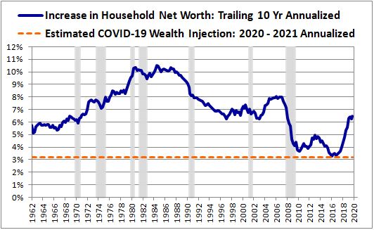
The government's addition of 3.2% per year in new financial wealth doesn't even reach that amount. Since the wealth will be added during a period in which overall wealth will be rising at a slower pace than normal—and in some sectors, actually falling—the final outcome could very well turn out to be a wash.
The wealth injected in the COVID-19 response looks even smaller when compared to the wealth that was injected during World War II. From the end of 1941 through the end of 1945, the government added roughly $200B of wealth to the private sector through deficit spending. It added that wealth onto a year-end 1941 private sector wealth level of $422B. The total increase was roughly 47%, more than seven times larger than the projected COVID-19 increase. Granted, the World War II wealth was injected over a 4-year period rather a 2-year period, but the time difference isn't likely to make much of a difference, given that the World War II economy wasn't investing to increase its peacetime productive capacity during the period.
Unfortunately, our technique of comparing the size of the wealth injection to the total amount of wealth in the system may not be accurate. The high level of wealth inequality in the system may render the comparison invalid, particularly for the COVID-19 wealth injection, which is targeted at the middle-income and lower-income segments of the economy. An addition of $7.5T to a total wealth value of $117T may only represent a 6.4% increase in that value, but it represents a much greater increase in the wealth levels of the middle-income and lower-income households that it's being delivered to. We should therefore expect it to have a greater stimulative impact.
For perspective on the degree of wealth inequality that currently exists in the U.S. economy, consider the pie chart below, which separates wealth ownership into three different wealth percentiles—top 10%, bottom 50%, and in-between—as of year-end 2019. The wealth percentile is shown in its respective color, and the percentage of total wealth owned by that percentile is shown in black (source: Distributional Financial Accounts):
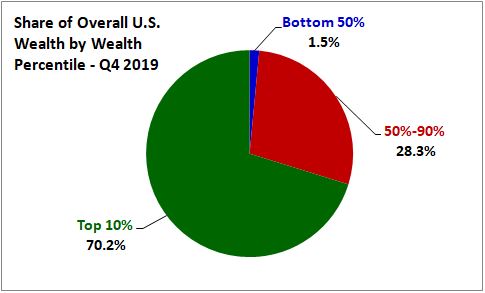
As you can see, the bottom 50% of the population only owns 1.5% of the wealth. If the $7.5T is delivered entirely to that segment, the effective wealth increase for the segment will come out to 427% (=6.4% / 1.5%), not 6.4%.
When we separate the economy into different income percentiles instead of wealth percentiles, we see a distribution of wealth ownership that is less skewed towards the high-end, but still strongly skewed in that direction. For context, the chart below shows the composition of the total net wealth owned by the bottom 20%, 20%-40%, 40%-60%, 60%-80%, 80%-99%, and the top 1% of income earners as of year-end 2019. The real estate, consumer durable and cash/bonds/other positions are expressed net of mortgage debt, consumer debt and other debt, respectively. The corporate equities position includes mutual fund and ETF holdings (source: Distributional Financial Accounts):
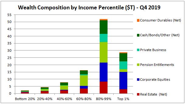
To put the chart in proper visual context, note that the column on the far right is the top 1%. It's not a separate quintile, yet it carries almost as much wealth as the bottom four quintiles combined, with the majority of the wealth taking the form of public and private equity.
To correct for the distortions that wealth inequality might introduce into the analysis, we need to connect wealth to actual spending, particularly for the segments of the economy that are going to receive the wealth injections. We can do this by introducing the concept of wealth velocity, defined as spending per unit of wealth. If we multiply the amount of wealth injected into each segment by its wealth velocity, we will be able to estimate the increases in spending that each segment will experience. Summing up the projected spending increases of all of the segments, we can then estimate the potential inflationary impact.
Readers will probably be familiar with the concept of money velocity, the total amount of nominal spending that occurs per unit of money in an economy per year. The problem with money velocity as a concept is that money is not the ultimate source of spending power. The ultimate source of spending power—both the ability to spend directly and, sometimes more importantly, the ability to borrow to spend—is wealth. Wealth is frequently held in the form of money, but it's also held in many other forms, the vast majority of which are readily convertible into money, given the liquidity provided by financial markets. Wealth velocity improves on money velocity by including these other forms in its denominator.
Segmented data on economic expenditures are only available for consumer expenditures, so for convenience in our calculations, we're going to specifically define wealth velocity as consumption spending per unit of wealth, which is the most important type of spending in a normal economy. Other types of spending, such as residential and corporate investment spending, can contribute to inflation, but they don't necessarily need to be included in the calculation, since we're only trying to estimate raw percentage increases. If we end up estimating that consumption spending will increase by a certain percentage in response to a given wealth injection, we can reasonably infer that the injection will bring about increases in magnitude similar to other forms of spending, assuming that historical relationships hold.
Almost all wealth in the economy is directly or indirectly owned by households, so we can formally define wealth velocity as annual personal consumption expenditures (PCE) divided by household net worth. The chart below shows the wealth velocity of the U.S. economy calculated under this definition from the 1st quarter of 1959 through year-end 2019 (source: FRED):
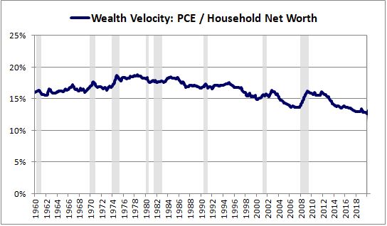
As of year-end 2019, the calculated wealth velocity for the trailing-twelve-month period was roughly 12.6%, indicating that households spent 12.6 cents annually on consumption for every dollar of net worth that they owned. The peak value for the velocity was roughly 19% in the second quarter of 1978. A significant portion of the difference between the current velocity and the peak velocity is attributable to valuation-driven increases in the economy's equity and real estate wealth. Equity and real estate assets are currently priced at much higher valuations than they were in the 1970's and early 1980's, and therefore the comparative amount of mark-to-market wealth in the economy—the denominator of the expression—is larger, pulling the expression down.
The relationship between wealth and spending is far from perfect. Increases in wealth tend to lead to increases in spending, but they don't necessarily lead to proportionate increases in spending, and they certainly don't have to lead to such increases, or to any increases at all. When wealth levels increase in ways that do not lead to proportionate increases in spending—as has occurred in the equity and real estate valuation boom of the last three decades—the mathematical result ends up being a drop in wealth velocity.25
Intuitively, we would expect wealth velocity to be lowest at the margin. In other words, if you have no wealth, and I gradually increase your wealth up to some end value, we would expect each incremental increase in your wealth up to that value to produce a smaller increase in your spending. At a certain point, your consumption demand will be fully quenched, and all of the incremental wealth that gets added will be withheld as savings. For this reason, wealth velocity as we've defined it—total consumption spending divided by total household net worth—will tend to overstate the actual wealth velocity occurring at the margin.
Because calculated wealth velocity overstates true wealth velocity at the margin, using it in our calculations will lead us to conclusions that are conservative. We will tend to overestimate the amount of spending that specific wealth injections will introduce, which is exactly what we should want to do, if our goal is to demonstrate that the economy can support those injections without experiencing significant inflation. We should want to be conservative, so that if we miss some important detail somewhere, we still have room to be right.
There's a sense in which our calculational technique can also lead to conclusions that are non-conservative. The non-conservatism arises from the fact that the wealth term in the denominator of the wealth velocity expression includes semi-illiquid forms of wealth that are costly and personally inconvenient to access—assets such as homes, 401K's, pensions, and stock holdings with embedded capital gains. The wealth that fiscal policy injects is not wealth of this type—it's straight liquidity that can be accessed at no financial or personal cost. It has a higher natural velocity than other forms of wealth, which could cause the technique to underestimate its spending impact. Different forms of wealth are fungible and are typically viewed as commensurate parts of a single overall account, so we should expect any impacts associated with this non-conservatism to be small.
To introduce the calculational technique, let's assume that the government is going to distribute the $7.5T COVID-19 wealth injection in a way that matches the economy's current uneven wealth distribution. Using the 12.6% wealth velocity as an estimate of the stimulative impact, we would expect the injection to translate into $945B (=$7.5T * 12.6%) of additional annual consumption spending. Prior to COVID-19, total annual consumption spending was roughly $14.7T, so the $945B increase would translate into a nominal consumption spending increase of 6.4% (=$945B / $14.7T). This number, of course, is the same number that we arrived at in our earlier calculation of the overall wealth change. The reasons are purely algebraic.
Importantly, the 6.4% number represents an estimate of the annual spending increase that would be introduced if the economy were to return to pre-pandemic wealth velocities. It doesn't capture the temporary effects of the pandemic itself, which will obviously pull down on spending over the near-term. A spending increase of 6.4% is a small increase, especially if introduced over a multi-year period, so if the number is accurate as an estimate, then we can be reasonably confident that the projected COVID-19 fiscal response, as a one-off injection, will not be significantly inflationary, not now and not in the future.
If we had applied the same calculational technique to the World War II wealth injection, we would have arrived at spending estimates that were more-or-less within range. Prior to the war, the U.S. economy's wealth velocity was roughly 19%. Over the course of the war, the government injected roughly $200B in deficit wealth. At the pre-war velocity, this wealth would have translated into an annual spending increase of roughly $38B (=19% * $200B) relative to pre-war levels, a 47% increase. The actual spending increase that occurred through year-end 1945 was roughly $39B, a 48% increase. Looking past the war, the actual spending increase that occurred through year-end 1946 was roughly $63B, a 77% increase. Given the importance of conservatism, we would have hoped for the technique to have overestimated the eventual spending increase rather than have underestimated it, but we have to remember that inflation was high in 1942 (~9%) and very high in 1946 (~18%), potentially distorting the nominal result.
The chart below shows the wealth velocity of the U.S. economy before, during, and after World War II. Note that the y-axis is zoomed in and starts at 16% (source: NIPA Table 2.4.5, Christensen et. al.):
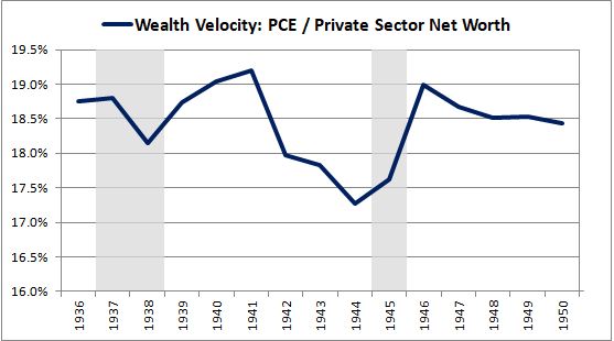
As you can see, the wealth velocity dropped during the war, but it eventually recovered. If you were to have proceeded on the blanket assumption that it would have stayed constant in the presence of the wealth injection, or that it would have eventually returned to its prior values after initially falling during the war, you would have been roughly correct. That assumption is the basis for the technique.
In the case of COVID-19, of course, the technique may not be accurate, since the economy's wealth distribution is highly uneven—more uneven than in the past. The injected wealth is not going to be distributed in accordance with that distribution, but is instead going to be distributed in a broad-based manner, with a focus on entities that need the money and that are likely to spend it. To arrive at accurate estimates, we will need to calculate wealth velocities for those entities and factor them into the overall result.
The chart below shows the wealth velocities of different income quintiles from 1989 through year-end 2019 (sources: Distributional Financial Accounts, BLS):
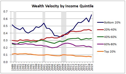
As expected, we see that lower-earning quintiles exhibit much higher wealth velocities than higher-earning quintiles. The bottom 20% of earners spend an amount equal to 65% of their net worth each year, whereas the top 20% of earners spend an amount equal to only 7% of their net worth. These numbers offer a different way of framing a point that is already well-understood: the poor have a much higher marginal propensity to spend than the rich. The point holds true for both income and wealth.
In the table below, we use the above wealth velocities to estimate the annual increases in total consumption spending that would be generated if the estimated $7.5T fiscal response were injected directly and entirely into the coffers of each of the five income quintiles. We also calculate an outcome for an "equal-weight" scenario in which the wealth is spread evenly across all five quintiles and a "COVID-19" scenario in which the wealth is spread out based on estimates derived from actual COVID-19 legislation26:
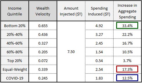
The results suggest that if all of the wealth were injected into the coffers of the bottom 20% of income earners, spending would rise by 33.4%. If the wealth were injected evenly across all of the income quintiles, spending would rise by 17.3%. If the wealth were injected based on allocation estimates derived from actual COVID-19 legislation, spending would rise by 12.5%.
Importantly, these numbers are based on pre-pandemic velocities—they do not reflect the temporary effects of the pandemic itself, which will obviously push down on spending over the short term. But at some point, the pandemic will pass, the job market will recover, and the world will return to normal. If the analysis proves to be conservative as intended, the numbers will represent upper-bound estimates of the spending increases that the injection will have introduced at that point, holding all other velocity-relevant variables—interest rates, tax rates, and so on—constant at pre-pandemic levels.
It's hard to know whether a recovered, post-pandemic U.S. economy will have the productive capacity to support a 12.5% increase in spending relative to baseline, so we can't rule out the possibility of a meaningful increase in inflationary pressure once the pandemic is resolved. If we were to experience such an increase, it wouldn't necessarily be a problem—it would simply mean that interest rates, and possibly tax rates, would have to rise relative to what they otherwise would have been.
Now, in our efforts to forecast the amount of inflationary pressure that the U.S. economy will experience, there are a number of relevant disinflationary factors that we need to consider. These include: (1) Income Inequality, (2) Anchored Inflation Expectations, (3) Cost-Push Deflation, (4) High Private Sector Debt Levels and (5) Aging Demographics. We discuss each factor separately below:
(1) Income Inequality: How did the economy get to a point where its existing wealth is distributed so unevenly? What caused it to get there? An important part of the answer can be found in the economy's income distribution, which is heavily skewed towards the high-end, more skewed than it has been in any prior period since the Great Depression. At present, the top two quintiles earn more than 75% of total pre-tax income while the bottom quintile earns less than 3% (source: BLS CE Survey, Mid-Year 2019):
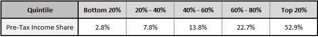
The economy's uneven income distribution matters to the analysis because, when spent, any new wealth that gets injected into the system is going to get re-filtered through that distribution. The wealth might start out in the hands of low-earners, but it's not going to stay in those hands. Low-earners are going to spend it. When they spend it, they're going to get less than 3% of it back as income. The stimulative exercise will then be over for them. The majority of the spending will turn into income for high-earners and for corporations, segments of the economy that have much lower marginal propensities to spend. Their withholding of the new wealth will attenuate the multiplicative process, muting the inflationary impact of the injection.
A similar point can be framed in terms of the reduced market power that low-skilled workers enjoy relative to high-skilled workers and to capital owners. This reduced power, which economists varyingly attribute to causes such as technological evolution, globalization, consolidation, and the decline of labor unions, makes it more difficult for low-skilled workers to extract income gains from the economy's spending gains. Those workers are important sources of spending in the economy. If they can't sufficiently extract income gains from the economy's spending gains, then inflationary chains of growth in income and spending are going to be significantly harder to sustainably induce.
As the injected wealth gets continually re-filtered through the economy's income distribution, it's going to retake the shape of that distribution. In that sense, our initial calculational strategy of assuming that the wealth would be distributed in accordance with the economy's existing wealth distribution might actually turn out to be the best option for forecasting outcomes. That strategy yielded an estimated spending increase of 6.4%, roughly half the increase shown in the table above.
Inequality in wealth and income is obviously a social problem to be lamented, but from a fiscal perspective, it's actually an advantage. It's what allows us to run aggressive fiscal interventions during crises without introducing longer-term inflationary pressures. The fact that the fiscal injections preferentially arrive and concentrate on the balance sheets of wealthy economic agents with low marginal propensities to spend is what prevents them from circulating in an inflationary manner.27
(2) Anchored Inflation Expectations: The role that expectations play in determining inflation outcomes is unclear, but if they're going to play any role in the current environment, it's likely to be a disinflationary role. Having lived through the subdued inflation environment of the last several decades, today's consumers and employers are not accustomed to accepting persistent increases in the prices and wages that they pay out. If conditions emerge that cause prices and wages to noticeably increase, consumers and employers are going to be more likely to interpret the increases as aberrations and resist them, seeking out better-priced substitutes and alternatives where available. Under sustained inflationary conditions, this propensity will shift, but in the near-term, we should expect it to help attenuate inflationary outcomes.
(3) Cost-Push Deflation: The economy may experience demand-pull inflation from the wealth injection, but this inflation could end up being offset by cost-push deflation arising from other sources. In recent years, the personal consumption category that has experienced the most cost-push deflation is goods. From 1995 to present, the price index of durable goods has fallen by over 40%, roughly 2% per year. Since 2011, the price index of nondurable goods has remained flat. As the chart below shows, these trends are not normal and represent significant historical anomalies (source: NIPA Table 2.4.4):
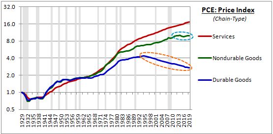
We can't know for certain why the trends have occurred, but we can speculate that the reason has something to do with the supply-side effects of technology and globalization. If those effects continue to put downward pressure on prices, they will help offset some of the inflation associated with the wealth injection.
The severe deflationary trend observed in the price indices of durable goods helps explain why the Fed has had such a difficult time achieving its 2% core PCE inflation target. Many people seem to think that the Fed's failure to reach the target is a recent phenomenon, but core PCE inflation has averaged below 2% in almost every multi-year period since the mid-1990's, the period when durable goods prices began to deflate (source: FRED):
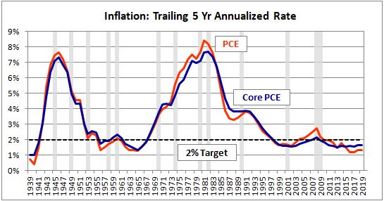
With respect to the above disinflationary trend, we can confidently project the technology-driven portion of the trend out into the future, but we have to be careful in projecting out other portions. Potential future weakness in the dollar and a potential transition into a process of de-globalization could give rise to the opposite trend--a trend towards cost-push inflation. Over the short-term, potential productivity impairments associated with COVID-19 could have a similar effect.
(4) High Private Sector Debt Levels: The U.S. private sector is currently carrying aggregate dollar-denominated debt equal to 141% of U.S. GDP.28 While this number is down from its 2008 peak of 155%, it's significantly higher than in any other period of history. High private sector debt levels increase the economy's natural withholding demand and also its sensitivity to interest rate increases. In comparison with the past, we should therefore expect the induced inflationary pressure of a given fiscal injection to be smaller and to require a less aggressive monetary policy response.
(5) Aging Demographics: We don't know for sure why inflation in developed economies has been as low as it has been in recent periods, but we have good reason to think that the answer has at least something to do with aging demographics. The economies that have experienced low inflation—Japan, Europe and the United States—share aging demographics as a common feature, and the severity of the disinflation has matched those demographics, with the oldest economy, Japan, experiencing the most disinflation, and the youngest economy, the United States, experiencing the least. The wealth velocity numbers used in the calculation already reflect the effects of an older U.S. population, so the point may not seem relevant. But over the next few years, the U.S. population is going to continue to get older. Wealth velocity numbers calculated on today's data are not going to capture the potential effect of that additional aging.
In considering the impacts of these disinflationary factors, my sense is that in the aftermath of the pandemic, the economy will be able to absorb the additional spending introduced by the wealth injection without experiencing significant inflationary pressure, especially if the injection turns out to be a one-time, pandemic-related event rather than a recurring feature of future fiscal policy. Interest rates will end up higher than they otherwise would have been, but not high enough to stress the financial system. Unfortunately, I cannot prove this conclusion to be true using the analytic methods described above. With a total boost to spending that could rise well into double-digit levels, it's possible that a stronger inflationary outcome could ensue, necessitating a monetary response that turns markets upside-down.
Section 3: Equity Market Valuation
When a government runs a deficit, it adds financial wealth to the private sector. The greater the preference to spend this wealth—whether on consumption or on investment in the real economy—the more it will affect profits and inflation, which we examined in the first two sections. The greater the preference to withhold the wealth—store it on a balance sheet—the more it will affect the valuations of existing assets, particularly equities. In this last section of the piece, I'm going to explore the dynamics of this process, quantifying its effects in the current market environment and showing how those effects can contribute to upside-down market outcomes.
The Market Impact of a Fiscal Injection
We can begin the analysis by walking through the dynamics of a simple wealth injection. Suppose that the government creates $1,000 and sends it to a specific individual person in the form of a check.
If the person is a marginal saver, then she will send the money to her brokerage firm, officially bringing it "into" the market, where she will use it to bid on financial assets. If she wants more equity in her portfolio, she will put in an order to buy equities. If she wants more fixed income, she will put in an order to buy fixed income. If she's not impressed by her present equity and fixed income options, if she senses that better opportunities will come later, then she will simply leave the money in the account as cash.
If the person is a marginal spender, then she will spend the money, probably into the corporate sector, which sells most of the goods and services on offer. The corporation that receives the proceeds of the spending will then disburse them in accordance with its liability profile. It may use them to boost wages, or hire new employees, or invest in new equipment, transferring the proceeds into the hands of entities with high marginal propensities to spend, who will likely spend them again, repeating the process. It may also send the proceeds out to its shareholders as dividends, or use them to buy back shares, delivering them into the hands of entities with high marginal propensities to save, where they will end up in the market, as they did above.
Each time the income proceeds get spent in the multiplication process, they will get filtered through the economy's existing income distribution. Because that distribution is lopsided, a large portion of the money will eventually end up in savings, where it will go "into" the market and bid on assets. The table below illustrates the estimated migration into savings using actual data for the U.S. economy (source: BLS):
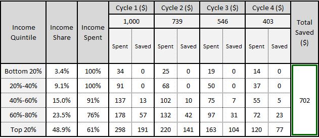
To walk through the table, we suppose that the government makes a fiscal injection of $1,000 into a single person's account and that the person spends all of the money. Neglecting taxes, $1,000 of income for the rest of the economy will then be generated. The $1,000 of income will get distributed in accordance with some distribution, which we approximate using the U.S. economy's actual current income distribution, shown in the second column of the table. The different quintiles of income have different marginal propensities to spend. To conservatively approximate these propensities, we take the percentage of total income spent by U.S. households in 2018, shown in the third column, and multiply it by the income received, allocating the leftovers to savings. We repeat the process through four subsequent cycles of multiplicative spending.
At the end of the four cycles, $702 of the initial $1,000 injection—roughly 70%—will have migrated into savings, with the rest waiting to be spent in the next cycle. The actual migration into savings will be larger, because the true marginal propensity to spend is lower than the conservative numbers that we've assigned.
A portion of the $702 in savings will be deployed into new investment, which will keep some of it flowing in spending, so that it stays out of the market. But new investment is more difficult to implement than the purchase of existing assets. It introduces greater capital and liquidity risk, and greater obstacles with respect to access. In most economic environments, the majority of the injection will therefore end up bidding on the existing asset universe—in particular, the segments of that universe that are expected to offer the best returns. In the current pandemic, those segments would include like the COVID-19-proof tech sector, which has become an endless destination for new money seeking a return.
To summarize the point, fiscal injections are market injections. Over time, they send financial wealth "into" financial markets, where it can bid on assets. This point holds true even when the injections are spent, because spending tends to migrate into savings over time, particularly in economies such as our own that exhibit high levels of income inequality and that offer limited opportunities for profitable new investment.
Buying and Selling Flow and the Like-for-Like Rule
Returning to the $1,000 fiscal injection, suppose that the person who receives it is bullish on the equity markets and decides to use it to buy equities. Her effort to buy equities will represent an instance of attempted buying flow. Given her preferences, the fiscal injection will have increased that flow, by however small an amount.
Apart from her specific case, as a sheer stock-flow statistical matter, an increase in the stock of an asset, i.e., its outstanding supply, will tend to translate into at least some increase in its attempted flow, because each unit of its supply will have some probability of attempting to flow in a given period. If that probability stays constant as the supply of the asset increases, then the amount of attempted flow emanating from the asset will increase as well. To illustrate with an example, if every dollar in an investor portfolio has a 0.5% probability of being used to purchase equities at current prices over a given time period, and if I increase the supply of dollars in portfolios by 100x without changing anything else in the system, I would expect to see a 50% (=0.5% * 100) increase in the raw quantity of dollars that end up bidding for equities at current prices.
As a rule, the actual buying and selling flows in an asset have to match at all times. If the attempted buying and selling flows in an asset do not match at a given price, then the price will change by whatever amount it needs to change by in order to get the attempted flows to match. The change might require the complex intermediation of market-makers and traders with differing time horizons, but it's essentially guaranteed to occur, since price is the only variable that can adjust to correct the imbalance.
The government's injection of money into the saver's account will increase the attempted buying flow occurring in the equity space, but will it increase the attempted selling flow? The answer is obviously no, as there's no reason to expect a fiscal injection to magically make people want to sell equities. The injection is therefore going to create an excess of attempted equity buying flow over selling flow, forcing a price increase. The actual change that registers from a $1,000 injection will surely be imperceptible, but its bias relative to the counterfactual will be in the upward direction. If we were to increase the injection amount to something extreme—say, $100T, to be delivered entirely into the hands of a single bullish investor who is eager to put the cash to work—we would definitely notice its effects.
The increase in attempted buying flow that emanates from the saver's efforts will represent a temporary condition that ceases after the desired transaction is executed. But the ensuing price increase can still hold, for two reasons:
(1) Supply Will Change in the Rest of the System: After the trade, there will be a greater supply of cash and a lesser supply of equity in the rest of the system, excluding the saver, who is no longer transacting. The increase in cash supply and the reduction in equity supply can lead to an increase in attempted buying flow and a decrease in attempted selling flow relative to the counterfactual, helping to sustain the price increase per the process described above.
(2) Prices are Sticky: Markets have memory and anchor to recent prices. If the price rises in response to the saver's buying efforts and stays risen for a sufficient period of time, market participants will come to view the new higher price as the "correct" price. They will viscerally interpret any significant downward deviation from that price as a potential buying opportunity, reacting to it in ways that help cement the earlier price increase.
To illustrate the point with an extreme example, suppose that instead of injecting $1,000 into the bullish saver's account, the government were to inject $15T, an amount roughly equal to half the U.S. equity market cap. Suppose that she were to follow through and use that money to buy out half the U.S. equity supply over the next 6 months, driving the S&P 500 to some crazy number—say, 6000. Once her transactions were completed, would the price fall back to its current level, 3300? No. If she is a tight holder of her position, then there will be half as many potential sellers as there were before, since the effective supply of the asset class will have been cut in half. Similarly, there will be $15T of new cash in the rest of the system, a large portion of which will be seeking to bid on the market. The shifts in supply caused by her action would help support the new equilibrium price. If the price fell—e.g., to a level of 5000, a 16% correction--people would think "Ooh, finally, a buying opportunity!" and would attempt to capitalize on it, supporting the price.
Now, in flow-imbalanced situations where the underlying values of the affected assets are like-for-like with present cash, i.e., well-defined and easy to fundamentally express in present cash terms, prices usually won't have to change by very much for a balance between attempted buying and selling flow to re-emerge. That's because a clear arbitrage opportunity will arise that will alter the fundamental attractiveness of buying and selling.
To illustrate with an example, consider the market for 3-month treasury bills (t-bills). As a security, a 3-month t-bill is almost identical to cash. If the government were to fiscally inject a large supply of cash—say, $15T—into the 3-month t-bill market, the amount of cash seeking to buy 3-month t-bills would likely increase, pushing up on prices. But prices wouldn't have to rise by very much to kill off the excess demand, because if the yield on the 3-month t-bill fell meaningfully below the yield on cash, there would no longer be any fundamental reason to want to hold it in lieu of cash.29 Everyone in the market would agree that cash was offering a higher return in exchange for the same credit and duration risk, and therefore everyone would seek to sell rather than buy. The attempted flows would quickly realign around the correct price, regardless of how much cash there was in the system to do the buying or how many t-bills there were that could be sold.
Now, when the underlying value of an asset is not like-for-like with present cash, i.e., not well-defined and not easy to fundamentally express in present cash terms, price changes aren't going to be able to create the same arbitrage opportunities, and therefore imbalances between attempted flows are going to exert stronger influences on price outcomes.
For an illustration, consider the example of a specific equity security, say Amazon ($AMZN). $AMZN is a stream of potential future cash flows that will be realized and paid out decades from now. Is there any clear or easy way to express the value of those cash flows in terms of present cash? No. To specify the present cash value of $AMZN's future cash flows, we would need an estimate of what those cash flows are going to be. Additionally, we would need to know the proper discount rate to apply to the estimate, which is the compensation that we get in exchange for accepting the risk that our estimate might be too high, and also for the risk that we might get stuck in the position with unpleasant mark-to-market losses, losses that could be quite large, if we end up buying too high. In the case of $AMZN, we can't confidently put numbers on any of those considerations, and therefore we can't confidently specify a correct price.
For this reason, as the price of an equity security such as $AMZN rises or falls in response to attempted flow imbalances, there's not going to be a point where an obvious arbitrage opportunity will emerge, or where the security will turn into an obvious buy or an obvious sell. The factors that eventually bring attempted flows in the security into balance are going to be much more crude and erratic, involving forces such as:
(1) Price Anchoring: The sense that the recent price of a security is the proper standard for assessing where the price should be and that deviations from that price require justification.
(2) Expectations of Mean-Reversion: The sense that what has fallen will eventually bounce back and that was has risen will eventually fall back down.
These forces are not always dominant in markets. They can easily be overcome by mechanical flows that are insensitive to price, or by forces that are price-sensitive in the opposite direction: reflexivity, momentum, trend extrapolation, and so on. In the case of excess buying demand, the ensuing price increase can cause buyers to become more fundamentally and technically optimistic than they already were, exacerbating the imbalance by drawing in additional interested buyers. Similarly, the price increase can cause sellers to become more relaxed and comfortable in their positions, less likely to feel a need to put those positions up for sale. When these forces dominate, prices have no choice but to deviate until the forces of anchoring and expected mean-reversion can regain traction.
Returning to the topic of fiscal injections, it's tempting to think that the financing method of a fiscal injection--whether the injection is financed through debt issuance or through money creation—will impact eventual market outcomes. But if we carefully think through the process, we will see that any potential impact will tend to be very small, particularly in the current environment.
The traditional process of fiscal spending consists of two separate events: (1) Spending and (2) Sterilization.
(1) Spending: The government directly spends money into the system. All of the previously described impacts, where the income multiplies and eventually lands as cash in the hands of savers that send it into financial markets, happen from this event. Pending their allocation preferences, the event will push up on the prices of all asset classes, to include equities.
(2) Sterilization: To keep the money supply constant, the government sells a bond to investors, removing an amount of money from the system equal to the amount that the spending event introduced. This event is its own separate event, involving separate market participants. It affects the market by creating additional supply and selling flow in government bonds, directly pulling down on the price of that one asset class.
The difference between debt-financed fiscal spending and money-financed fiscal spending lies in the presence of the second event, sterilization. In debt-financed fiscal spending, sterilization is a core part of the process. In money-financed fiscal spending, it's either left out of the process or fully undone through the reverse process, quantitative easing, whereby the central bank uses newly-issued money to purchase government bonds.
The spending event happens in both cases, and pushes up on the price of equities relative to the counterfactual. Does the sterilization event pull down on the price of equities in a similar manner? If the answer were yes, then, on a cumulative basis, debt-financed spending would be less buoyant to equity prices than money-financed spending.
The argument for why we should expect sterilization to pull down on equity prices is that the government is soaking up money by selling a bond that competes with other asset classes for buyers. To draw in buyers, the government will presumably have to sell the bond at a yield that's attractive on a relative basis. In selling the bond at an attractive yield, will the government draw buying interest from equity holders, inducing them to sell some of their equity positions to raise cash so that they can take advantage of the opportunity?
The answer would seem to be no, at least not to any noticeable degree. The equity market is distinct from the bond market—there's no reason to think that a sale of supply on attractive terms in one market will perturb and draw money out of the other. More importantly, the like-for-like rule suggests that the money that ends up purchasing the bonds will be significantly more likely to come out of existing cash and fixed income positions than to come out of existing equity positions. As the yields on the bonds are increased to attract buyers, a clear fundamental arbitrage is going to emerge between the bonds and comparable cash and fixed income assets long before any such arbitrage will emerge between the bonds and equities, a fundamentally different and incomparable asset class. This point is particularly true in the current environment, where cash and fixed income yield nothing. Offering a 1% yield on the bonds will be enough to make the entire current cash and fixed income market want to buy in, but it's not going to be enough to draw any meaningful interest at all from equity investors, who have chosen to partake in a fundamentally different risk-reward proposition.
Another useful way to frame the point is in terms of portfolio allocations. When the government engages in fiscal spending, the net effect of its action is to inject assets into investor portfolios—either government bonds or cash, depending on how the spending is financed. The injection will ultimately reduce investor allocations to all other asset classes, including equities. Unless, by coincidence, this reduction happens to be wanted by investors, it's going to put upward pressure on prices, as investors attempt to get their allocations back to where they had them before the injection.
The difference between an injection of cash and an injection of government bonds is unlikely to make much difference to this outcome since cash and government bonds are extremely similar as asset classes. They've been rendered especially similar in the current environment, where Fed signaling and quantitative easing—the reverse of the sterilization process described above—have pushed the yields on government bonds almost all the way down to zero, the same yield as cash. If the government wanted to, it could use quantitative easing to convert all of its bonds into cash. Outside of possible placebo effects, the difference would make little difference to equity prices since those bonds are already essentially functioning as cash in portfolios.
The Average Investor Allocation to Equity
When presented with an investment menu consisting of different asset classes with different risk-dynamics and different expected returns, different market participants are going to have different allocation preferences with respect to each asset class. Some investors will prefer to allocate their portfolios primarily to equities, while others will prefer to allocate their portfolios primarily to cash and bonds.
Looking at a market in its entirety, we can speak of an "average" allocation preference, which would simply be the value-weighted average of the allocation preferences of the individual participants. If you and I are equally-sized players that comprise the entire market, and if you want a portfolio consisting of 70% equity and 30% cash and bonds, while I want a portfolio consisting of 70% cash and bonds and 30% equity, then our "average" allocation preference will be 50% to each.
We can roughly quantify the "average" allocation preference of a market at current prices by counting up the supply—i.e., the aggregate market value, defined as price times shares outstanding—of the asset classes inside it. That supply is the total "amount" of the asset class in existence, and also the total "amount" that is theoretically available for investors to allocate their wealth into.
Recall that investors, as a group, have to hold every unit of every asset in the market at all times. If investors want to hold more of an asset at a given price than the existing supply of that asset can support, then they will transact accordingly, individually seeking to buy more of the asset and bidding up its price in the process. The struggle to get more of the asset will continue until the investors collectively get to their desired allocations. They themselves will make it possible to get to those allocations because the rising price of the asset will lead to a rising market value and therefore a rising supply to allocate into. The same principle applies in reverse—by attempting to sell asset classes that they want to hold less of, investors will shrink the supply of those asset classes and make it possible for everyone to hold smaller amounts of them.
We can use the chart below, taken from the 2019 Japan Flow of Funds report, as an approximation of the average allocation preference of U.S., Japanese, and European households (source: BOJ):
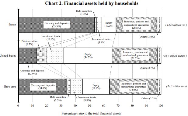
The asset classes are divided into currency and deposits, debt securities, investment trusts, insurance claims, pension claims, standardized guarantee claims, and finally, equities. Note that the equity allocation includes allocations to foreign equities in addition to domestic shares.
If you look closely at the chart, you will notice that American households have a strong preference for holding equities, much stronger than the preferences of Japanese and European households. This fact is surprising because cash and bonds in Japan and Europe offer negative yields, a key difference in comparison with the United States, which respects the zero-lower bound. Despite the negative cash yields in Europe and Japan, investors in those countries have priced their equity markets to offer strong earnings yields, higher than in the United States, even after adjusting for sector differences. The inefficiency is puzzling on both ends.
Why don't European and Japanese households take advantage of the enormous premium over cash and bonds that their equities appear to be offering? Why don't they bid up the prices of those equities, driving up the overall allocation to equity? The answer is a mystery; it likely has something to do with differences in the respective financial cultures and in the lived experiences of market participants of the different countries. At least in Japan, the investor experience has been nowhere near as rewarding as it's been in the United States. Given the deep equity preference of U.S. investors, it's scary to think about what would happen if the U.S. central bank were to impose a meaningful negative interest rate on cash. If the penalty were actually passed onto depositors, the panicked stock market buying frenzy that would ensue would be a sight to see.
Unfortunately, we can't use the quoted equity allocation above as an approximation of the total relative supply of equity in the respective nations because other entities in the chart—e.g., investment trusts, insurance companies, pension funds, and so on—also own portions of the equity universe. But if we do some leg work in the Japan Flow of Funds, we can conservatively account for equity contained in those other locations. We end up with the following chart, which simplifies the allocation into two categories: equity, and cash and bonds (and loans, etc.):
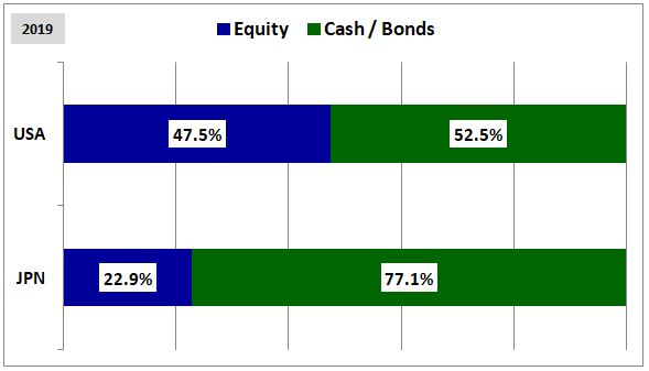
With indirect equity ownership added to the total, Japanese Households have less than half the equity exposure of U.S. households. Importantly, this difference isn't the result of a lack of potential Japanese equity supply—Japanese equities are cheap, with plenty of room to expand in supply via price increases. And if Japanese households don't like their own equities at current prices, they're free to buy U.S. and European equities. Instead, they've chosen to hold the majority of their assets in fixed income instruments at zero or negative yields.
The Upside-Down Portfolio Effects of the COVID-19 Deficits
Over time, as the COVID-19 deficits collect in the hands of savers, they will end up functioning as direct injections of cash and treasury bonds into investor portfolios. These injections, which will represent insertions of new wealth rather than alterations in the composition of existing wealth, will raise allocations to cash and treasury bonds and reduce allocations to every other asset class—most notably, equities.
Do investors actually want to have their allocations to equities reduced in this way, replaced on a percentage basis with cash and bonds? Probably not, especially with the Fed having just lowered interest rates to zero. But they don't have much choice in the matter; if they don't want to accept the reduced allocations, then their only available option, outside of investing in new companies or in companies that are diluting, will be to push up on the prices and valuations of existing shares.
The chart below shows the existing supply of equities (blue) and all forms of debt (varying shades of green) in the dollar-denominated asset universe from 1946 through year-end 2019, expressed as a percentage of the total supply (source: FRED):
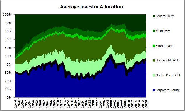
Notice that we've left cash, as an asset class, out of the chart. The reason that we've left it out is that it's already fully captured in the debt assets contained in the chart. Cash is what private investors end up holding when banks—to include the central bank—hold debt assets on their balance sheets, as investments for themselves. The banks effectively take the debt assets out of investor circulation and replace it with cash that goes into investor portfolios.
To illustrate with an example, suppose that a commercial bank issues a loan to a corporation and decides to hold that loan as an investment on its balance sheet. Because the bank is holding the loan, it won't show up as a debt asset in investor portfolios. Instead, it will show up as cash, because investors will have to hold the cash—i.e., the bank deposit—that gets created by the loan and spent into the economy. The bank's decision to hold the loan will simply change the form in which it shows up inside portfolios—from debt into cash.
Similarly, if the central bank decides to buy a bond from investors in an open market operation, the bond will get taken out of investor circulation. But it won't fully disappear from investor portfolios because it will get replaced by the cash that the central bank "prints" to make the purchase, cash that the seller of the bond will now have to hold in his portfolio. The central bank's action will again change the form of the underlying holding--from debt into cash.
Recognizing this point, we can interpret the green portion of the chart above, as either (1) bonds or (2) bonds that the banking system has effectively converted into cash. In the current environment, there's not much of a difference between these two categorizations, because everything essentially yields what cash currently yields—nothing. With the exception of a small sliver of risky corporate bonds, foreign bonds, and mortgage-backed securities, the only portion of the above chart that stands out as having any potential to deliver a meaningful long-term fundamental return is the blue portion, the equity portion.
Is there a shortage of equity in the market? Historically speaking, the answer is no. Neglecting the effects of COVID-19 debt issuance, equities constitute roughly 46% of the dollar-denominated asset universe. That number is in the top 5th percentile of all historical readings. Relative to the size of the U.S. asset market, there has rarely been a greater supply of equity available for investors to deploy their savings into.
If there's a shortage of anything, it's a shortage of available return. With the exceptions of equities and high-yield bonds, none of the assets in the current investment universe are priced to offer any return. A return shortage is to be expected in a low-potential-growth environment where interest rates have been set at zero and are expected to be kept near zero for a very long period of time. Indeed, that's one of the purposes of low-interest rate policy—to stimulate investment, i.e., the creation of new assets, by making the returns on existing assets less attractive.
When the COVID-19 deficits eventually land in investor portfolios as new wealth, the government will have effectively injected $7.5T worth of zero-yield or near-zero-yield instruments into those portfolios, increasing the realized allocation to cash and bonds and reducing the realized allocation to equity. If the entire $7.5T were injected today, the current investor allocation to equity would fall to roughly 42.2%, compared to a 2019 year-end value of 46.2%. At the time of this writing, the S&P 500 is roughly unchanged for the year, so the COVID-19 fiscal response will have had the effect of forcibly reducing the average equity allocation by 4%—probably more in the final analysis (source: FRED + author extrapolations)30:
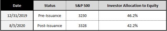
We highlight the magnitude of the reduction in the chart below:

Do investors actually want a 4% reduction in their allocation to equities? If not, then in the absence of new equity issuance, their only option will be to fight with each other over the existing supply, which will have grown more scarce on a relative basis. If they continue in this fight, they will end up inflating prices and increasing the supply, making it possible for their prior allocation preferences to be collectively achieved.31
Valuation acts in opposition to this process. If investors are sensitive to valuation, rising prices will reduce their desire to allocate to equities. But it's difficult for valuation to gain traction as a consideration in the current environment. The relevant value proposition that investors have to consider is an awkward proposition that pits positive-but-historically-depressed earnings yields in equities against zero yields in everything else. Rising equity valuations cannot easily shift the balance of that proposition for at least two reasons. First, equities can produce attractive returns even when purchased at elevated valuations, provided that they stay at those valuations—and in the current case, they very well might. Second, the alternative proposition—earning a negative real return for an indefinite period of time while others continue to make money--is simply unacceptable to many investors.
We refer to this logic as the logic of TINA—"There is No Alternative." The logic is sound, but it has limitations. Equities aren't going to rise to infinity—an earnings yield of zero--simply because the competition is yielding zero. As equities become more expensive, they become more "needy", more sensitive to declines in buyer enthusiasm. Their neediness and dependence on continued buyer enthusiasm increases their potential for inflicting losses.
To illustrate, imagine that you are in a two-asset market where one asset, cash, earns nothing forever, and the other asset, an equity stream, earns $1 a year forever, with a portion of that amount paid out as a dividend and a portion reinvested to generate future growth. If you buy the equity stream for $10—an earnings yield of 10%—and the enthusiasm of buyers subsequently wanes, you won't need to sell at a loss. If the price falls, it's not a big deal, because the 10% yield that you be will earning on the investment is intrinsically worth the temporary loss of access to your money. All you will have to do is wait and let the earnings accumulate, either as dividends that get paid out to you or as investments that compound. Over the long-term, you will end up doing very well, regardless of where the market decides to take the price.
But now suppose that the price gets pushed up in a TINA chase to $100—an earnings yield of 1%. If you buy at that price, you're going to have to remain laser-focused on the market's subsequent response, keeping the position on a short leash and rapidly exiting if buyer enthusiasm starts to wane, because the 1% earnings yield that you're going to be accruing is nowhere near enough to compensate you for the loss of access to your money, which is what you will have to endure if the price falls appreciably from where it currently is. If the market decides that it wants to assign a 20 P/E ratio to the security instead of a 100 P/E ratio, the price is going to fall by 80%. You're going to have to wait a full 80 years to get your money back in earnings. Will the wait be worth the 1% spread over cash that you will have locked in? Absolutely not, which is why you're going to have to pay close attention and make sure that you don't get stuck in that kind of a situation.
In the same way that you are going to be more sensitive to drawdown risk as a buyer at elevated valuations, everyone else in the market is going to be more sensitive as well, which will make the prices themselves more sensitive, and the investments more risky.
Ultimately, the only way that a market can be stable is if everyone is more-or-less happy with what they are holding—willing to transact, but not feeling an urgent need to do so. In the hypothetical market above, is it going to be possible for everyone to be happy with what they are holding? Definitely not. If the equity price in that market is stable or rising, the underinvested individuals earning nothing in cash are going to be unhappy. They will want more equity and will chase prices higher until some counterbalancing disincentive emerges to discourage them, such as the disincentive of a needy, shaky, creaky market that looks and feels more expensive than it deserves to be. If the equity price is falling, then overinvested individuals taking losses in equities will be unhappy, and will chase prices lower in pursuit of the safety of cash, until prices get cheap enough to make the securities attractive as investments for their own sake, because the underlying cash flows are attractive, regardless of the price that they can be sold for.
In the end, TINA markets are guaranteed to be difficult and frustrating for large numbers of people. The problem of how to properly invest in them has no easy solution. Chasing ultra-expensive assets, nervously supervising them in the hopes that you haven't top-ticked them, is stressful and unpleasant. But so is waiting on the sidelines earning negative real returns while everyone else makes money. Time is not on your side in that effort.
Returning to the subject of the current equity market, on the assumption that investors display zero sensitivity to valuation and invest entirely based on a pre-determined asset allocation preference, we can quantify the exact impact that the COVID-19 deficits would be expected to have on prices, if they found their way into markets. We simply assume that investors would bid up on the price of equity until their pre-pandemic allocation to equity was restored. To restore that allocation amid the COVID-19 debt issuance, the market would have to rise by roughly 18%, from its price at the time of the writing of this piece, roughly 3327, to a final price of roughly 3900, a forward 2-yr GAAP price-earnings ratio of 26 times.
In exploring the supply-driven effects that fiscal policy can have on asset prices and valuations, we've once again arrived at a classic upside-down outcome. An event occurs that damages the economy, forcing extreme issuance of zero-yield government debt, the presence of which pushes down on average equity allocations and up on equity prices and valuations, contrary to the assumed effect of the damage itself.
1 As a legal matter in the U.S., negative interest rates are incompatible with the language of Section 19 of the Federal Reserve Act and would likely require congressional passage of an amendment to the act.
2 To arrive at this number, we start with the Congressional Budget Office's current CY 2020 and CY 2021 deficit estimates of $3.7T and $2.1T based on laws currently passed and add an additional $1T and $0.7T to reflect further stimulus measures that are likely to be implemented.
3 Across the majority of the piece, whenever I use the term "wealth", I'm going to be referring to net wealth, which subtracts out liabilities. Sometimes, however, I'm going to use the term in a way that does not subtract out liabilities. Readers concerned with the distinction will be able to tell the difference.
4 We use the example of 1959 to illustrate the relationship because it was a year in which the current account balance was roughly zero, allowing us to ignore the foreign sector.
5 This increase does not include increases associated with changes in the market valuations of existing assets.
6 If the original deficit spender ends up being the one to withhold it, then he's no longer a deficit spender for the given period. He got back all of his spending as income, therefore he didn't spend in excess of his income.
7 This investment includes foreign corporate investment into the country. We're not going to separate foreign corporate investment out as a separate term because it's small relative to other types of investment and because it's already captured in the corporate investment term in NIPA table 5.1 that we're going to use to fill in the equation.
8 Because the corporate investment term includes the investments of foreign corporations into the country, it overstates the investment of the country's national corporations, which is what the equation is attempting to track. The overstatement is not a problem, however, because it's exactly cancelled out by the fact that the current account balance does not include the investments of foreign corporations into the country, and therefore understates the actual income surplus generated through foreign interactions by the same amount.
9 Share buybacks have the same economic and financial effects as dividends, but they don't matter to the equation because they don't explicitly affect any of its terms, They don't affect the investment term because they don't lead to the creation of new wealth. They don't affect the dividend term because they don't reduce the existing wealth contained in the corporate sector. When a corporation buys back shares, it loses the cash used in the purchase, but it gains an equivalently-valued asset—the purchased shares—in return. Its overall wealth therefore stays constant.
10 We use Gross National Product rather than Gross Domestic Product because the relevant corporate profit term in the equation is the profit of national U.S. corporations operating within and outside the U.S. The foreign profits of those corporations are not captured in Gross Domestic Product.
11 Households can save by buying existing assets—homes, shares in publicly-traded companies, etc. —but this doesn't solve the problem because all they're doing when they buy existing assets is swapping positions with other households in the system. Whoever sells to them ends up in their place, with a decision to make about what to do with the money received from the sale.
12 The original Kalecki-Levy equation, which we showed in (8) above, fails to fully capture the quantity of deficit spending that occurred during World War II. That's because it represents the government's participation through a "government saving" term. Saving is a sum of two terms—a withholding term (a negative term in this case, because the government is deficit spending) and an investment term (a positive term that offsets the withholding term). For governments, the investment term is usually negligible, but in the case of World War II, it was very large, roughly 12% of GNP per year, reflecting the large amount of war-related construction and research that the government was funding. Reported annual government saving during World War II, which came out to approximately -14% of GNP, includes a positive 12% offset from this investment. The actual amount that the government borrowed to fund consumption and investment was more than 26% of GNP, higher than any other year in history. Part of the benefit of reformulating the Kalecki-Levy equation in terms of borrowing rather than saving is that doing so helps us capture and better appreciate the enormity of the government's intervention during the war.
13 The BEA defines "personal saving" as the percentage of disposable income leftover after taxes and expenditures. It offers a rough proxy for "withholding" as we've defined the term.
14 In contemplating this point, readers might think that since the entirety of an investment will eventually be depreciated, the schedule shouldn't matter. Whether you understate an investment's useful life and pull its depreciation charges forward, or you overstate its useful life and push its depreciation charges back, the same overall expense will eventually be incurred. But this interpretation misses the fact that the economic aggregates that depreciation expenses get subtracted from—investment and revenue—are perpetually growing over time, both nominally and in real terms. If you understate the useful life and pull future depreciation expenses forward, you will end up subtracting them from smaller investment and revenue numbers that are closer to the present, distorting the net numbers in the downward direction. Conversely, if you overstate the useful life and push the present depreciation expenses back, you will end up subtracting them from larger investment and revenue numbers that are farther out into the future, distorting the net numbers in the upward direction. If you want an accurate picture of the trajectory of net investment and net revenue over time, you need to specify the useful life correctly, based on what the true useful life actually is.
15 These measures include the Family First Coronavirus Relief Act (FFCRA), the Coronavirus Aid, Relief and Economic Security (CARES) Act, the PPP, and Health Care Enhancement Act (PPPHCA), and future packages yet to be passed in law.
16 An accounting mismatch may emerge in this context as the costs that have to be undertaken to win approval for loan forgiveness are current costs, whereas the forgiveness will only be recognizable from an accounting perspective in the future, when it's approved—possibly years into the future.
17 I do not assign any increase to the state and local government deficit because the actual increase is likely to be subsumed by the federal increase, given that a relevant portion of the federal outlay is expected to be used to provide financial aid to state and local governments.
18 The earned disposable income numbers consist of wages, salaries, company benefits, proprietor income, dividend income, interest income, social security income, medicare, and veteran benefits, net of taxes, interest expense and contributions to social security and medicare. Importantly, the numbers excludes unemployment benefits, medicaid and other forms of government assistance.
19 The prospect of fiscal targeting offers an interesting argument in favor of market cap weighting. Of all possible index weighting schemes, market cap weighting is the scheme that most closely mimics the composition of the overall economy. If the goal is to build a portfolio whose revenue tracks the revenue of the overall economy (the variable being insured in the targeting regime), there's no better scheme to use.
20 We have to ignore possible boosts to profits from currency-depreciation-driven improvements in the current account balance because those improvements would ultimately arrive in the form of increased foreign spending into the corporate sector, which would imply a reduction in government deficit spending, since less deficit spending would then be needed to achieve the government's growth target.
21 See Christensen and Jorgenson, “US Income, Saving and Wealth, 1929-1969.” Review of Income and Wealth 19, no. 4 (1973): 329-362.
22 Interest rates at these levels might be necessary to hold back the spending and the associated inflation pressure that the wealth injection would otherwise introduce, but if they make it extremely expensive to borrow for the purpose of investment, then they could still introduce cost-push inflation pressure from the supply-side. They could also introduce cost-push inflation pressure by creating income streams that are sufficient to allow portions of the population to sustainably retire on the newly-injected wealth, shrinking the available labor supply in the system.
23 Tax increases would be necessary because the real interest rate needed to keep inflation on target would be substantially higher than the economy's real growth rate, making deficits unsustainable in the long run. Mathematically, the equilibrium Debt-to-GDP ratio for an economy with a primary (pre-interest) deficit d, a real interest rate i, and a real GDP growth rate g, equals d / (g - i). When i rises above g, the equation blows up, which means that any sustained primary deficit ends up leading to an endless rise in the Debt-to-GDP ratio. An endless rise in the Debt-to-GDP ratio is an endless rise in the Wealth-to-GDP ratio, a rise that no economy can support. If the rise is ever going to stop under the specified conditions, the primary deficit will have to be closed. Its closure will presumably necessitate tax increases.
24 Considerations related to asset supply, discussed in Section 3 of the piece, would help mitigate the drop.
25 The relationship can also go the other way—increases in spending can lead to increases in income which, at constant valuations, can lead to increases in the mark-to-market values of the real income-earning assets that receive the increased income.
26 To arrive at the COVID-19 estimate, we project out the $600 per week unemployment insurance enhancement through the end of the year and assume that it will be injected into the lowest income quintile. We take the remainder of the injection and distribute it on an equal-weighted basis or to the top 20% based on whether it is expected to be allocated to households or to the corporate sector.
27 There's a loose analogy here to the costs and benefits that the U.S. enjoys in being the world's reserve currency. The cost is that we end up with an overvalued currency and a depressed export sector. But the benefit is that when we aggressively print that currency and spend it to deal with economic problems, it tends to end up in the hands of foreign entities that are eager to hold it, mitigating the decline in foreign exchange value that it would otherwise suffer.
28 In the current context, we define the private sector as U.S. households, U.S. corporations, U.S. state and local governments, and the rest of the world.
29 The only potential reason to want to hold it would be to avoid the counterparty risk that comes with holding large amounts of FDIC-uninsured cash at a depository institution.
30 The quoted 42.2% number includes the noticeable effect of COVID-19-related nonfinancial corporate debt issuance through the end of the 1st quarter as well as the effect of equity float shrinkage from 1st quarter share buybacks, most of which occurred before the pandemic took hold. The number does not include the potentially noticeable effects of COVID-19-related foreign debt issuance, municipal debt issuance, nonfinancial corporate debt issuance (think: PPP), or equity dilution after the 1st quarter.
31 In theory, as equities become more expensive, their supply should grow through increased share sales. But in practice, this doesn't seem to happen, at least not to the extent that it would need to happen in order to quench the imbalances. For existing companies, the relationship between valuation and share sales tends to be the opposite of what theory would predict—companies tend to sell shares at depressed valuations during downturns, when they need to sell, and rarely during expansions, when sidelined investors seeking greater equity allocations would want them to.
General Legal Disclosures & Hypothetical and/or Backtested Results Disclaimer
The material contained herein is intended as a general market commentary. Opinions expressed herein are solely those of O’Shaughnessy Asset Management, LLC and may differ from those of your broker or investment firm.
Please remember that past performance may not be indicative of future results. Different types of investments involve varying degrees of risk, and there can be no assurance that the future performance of any specific investment, investment strategy, or product (including the investments and/or investment strategies recommended or undertaken by O’Shaughnessy Asset Management, LLC), or any non-investment related content, made reference to directly or indirectly in this piece will be profitable, equal any corresponding indicated historical performance level(s), be suitable for your portfolio or individual situation, or prove successful. Due to various factors, including changing market conditions and/or applicable laws, the content may no longer be reflective of current opinions or positions. Moreover, you should not assume that any discussion or information contained in this piece serves as the receipt of, or as a substitute for, personalized investment advice from O’Shaughnessy Asset Management, LLC. Any individual account performance information reflects the reinvestment of dividends (to the extent applicable), and is net of applicable transaction fees, O’Shaughnessy Asset Management, LLC’s investment management fee (if debited directly from the account), and any other related account expenses. Account information has been compiled solely by O’Shaughnessy Asset Management, LLC, has not been independently verified, and does not reflect the impact of taxes on non-qualified accounts. In preparing this report, O’Shaughnessy Asset Management, LLC has relied upon information provided by the account custodian. Please defer to formal tax documents received from the account custodian for cost basis and tax reporting purposes. Please remember to contact O’Shaughnessy Asset Management, LLC, in writing, if there are any changes in your personal/financial situation or investment objectives for the purpose of reviewing/evaluating/revising our previous recommendations and/or services, or if you want to impose, add, or modify any reasonable restrictions to our investment advisory services. Please Note: Unless you advise, in writing, to the contrary, we will assume that there are no restrictions on our services, other than to manage the account in accordance with your designated investment objective. Please Also Note: Please compare this statement with account statements received from the account custodian. The account custodian does not verify the accuracy of the advisory fee calculation. Please advise us if you have not been receiving monthly statements from the account custodian. Historical performance results for investment indices and/or categories have been provided for general comparison purposes only, and generally do not reflect the deduction of transaction and/or custodial charges, the deduction of an investment management fee, nor the impact of taxes, the incurrence of which would have the effect of decreasing historical performance results. It should not be assumed that your account holdings correspond directly to any comparative indices. To the extent that a reader has any questions regarding the applicability of any specific issue discussed above to his/her individual situation, he/she is encouraged to consult with the professional advisor of his/her choosing. O’Shaughnessy Asset Management, LLC is neither a law firm nor a certified public accounting firm and no portion of the newsletter content should be construed as legal or accounting advice. A copy of the O’Shaughnessy Asset Management, LLC’s current written disclosure statement discussing our advisory services and fees is available upon request.
Hypothetical performance results shown on the preceding pages are backtested and do not represent the performance of any account managed by OSAM, but were achieved by means of the retroactive application of each of the previously referenced models, certain aspects of which may have been designed with the benefit of hindsight.
The hypothetical backtested performance does not represent the results of actual trading using client assets nor decision-making during the period and does not and is not intended to indicate the past performance or future performance of any account or investment strategy managed by OSAM. If actual accounts had been managed throughout the period, ongoing research might have resulted in changes to the strategy which might have altered returns. The performance of any account or investment strategy managed by OSAM will differ from the hypothetical backtested performance results for each factor shown herein for a number of reasons, including without limitation the following:
▪ Although OSAM may consider from time to time one or more of the factors noted herein in managing any account, it may not consider all or any of such factors. OSAM may (and will) from time to time consider factors in addition to those noted herein in managing any account.
▪ OSAM may rebalance an account more frequently or less frequently than annually and at times other than presented herein.
▪ OSAM may from time to time manage an account by using non-quantitative, subjective investment management methodologies in conjunction with the application of factors.
▪ The hypothetical backtested performance results assume full investment, whereas an account managed by OSAM may have a positive cash position upon rebalance. Had the hypothetical backtested performance results included a positive cash position, the results would have been different and generally would have been lower.
▪ The hypothetical backtested performance results for each factor do not reflect any transaction costs of buying and selling securities, investment management fees (including without limitation management fees and performance fees), custody and other costs, or taxes – all of which would be incurred by an investor in any account managed by OSAM. If such costs and fees were reflected, the hypothetical backtested performance results would be lower.
▪ The hypothetical performance does not reflect the reinvestment of dividends and distributions therefrom, interest, capital gains and withholding taxes.
▪ Accounts managed by OSAM are subject to additions and redemptions of assets under management, which may positively or negatively affect performance depending generally upon the timing of such events in relation to the market’s direction.
▪ Simulated returns may be dependent on the market and economic conditions that existed during the period. Future market or economic conditions can adversely affect the returns.