ML & Investing Part 1: From Linear Regression to Ensembles of Decision Stumps
By Kevin Zatloukal
December 2018
Introduction
The idea of applying machine learning to finance and investing has become a popular topic of discussion recently, and for good reason. As its use becomes widespread, machine learning (ML) has the potential to change almost every part of society, both by automating routine activities and by improving performance in difficult activities. In all likelihood, investing will be no exception.
While the accomplishments of machine learning are capturing the headlines, the goal of this article is not to dazzle you with those accomplishments or awe you with the mathematical sophistication of some ML methods. To the contrary, our goal is to demonstrate machine learning techniques that not only are simple but also greatly extend the power of familiar tools. In particular, we will describe ensembles of decision stumps and discuss how to view them as a generalization of linear regression that can capture some non-linear patterns in data.
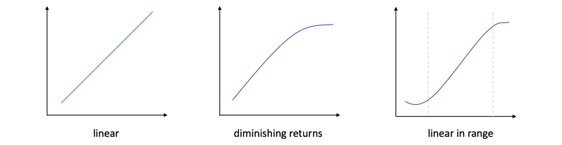
This additional explanatory power is important because linear relationships are rare in nature. The method we will discuss can still capture linear relationships, like the one shown on the left below, but, in addition, can accurately describe relationships that exhibit non-linearity such as diminishing returns or relationships that are linear but only hold within a limited range of values, as in the other two plots. Later in this article, we will see these types of situations in familiar investing examples.
You might worry that using ensembles of decision stumps will require drastic changes to your process for analyzing data, but fortunately, this is not the case. There is essentially just one change we need to make to our process, which we will highlight below. Furthermore, that change not only allows us to use ensembles of decision stumps, but also puts the full collection of machine learning tools at our disposal, should we desire to use them.
A Gentle Introduction to Machine Learning
The only background we will assume is a basic knowledge of linear regression. That is a great place for us to start because linear regression is itself a machine learning algorithm. In this section, we will use linear regression as an example to explain some machine learning terminology and highlight where the machine learning perspective differs from that of traditional statistics.
Linear regression is a basic algorithm for solving a supervised learning problem. The data given to us in this problem are a collection of labelled examples, like these:
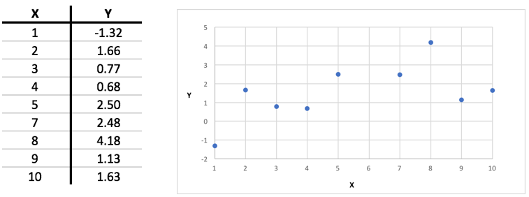
The goal here is to figure out, from the given examples, a way to predict the labels (the Ys) on new examples (new Xs) as accurately as possible.
In almost every case, the data given to us in a supervised learning problem will describe each example not with a single "X" value but instead with many numbers. Even the simplest example we will look at later in this article includes two different Xs for each example, along with the label Y:
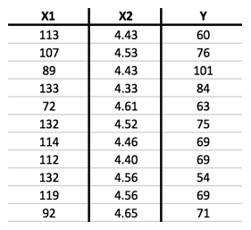
In ML terminology, the different Xs are called features.
A solution to the supervised learning problem gives us a way of guessing the label of a new example, when given only its features as input. Linear regression solves this problem by finding the "best fit line" for the given examples. With the collection of examples plotted above, the best fit line looks like this:
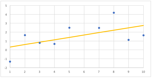
With that line in hand, we can guess the label for a new example just by finding the height of the line at that X position. At X=6, for example, we would guess a label around 1.6:
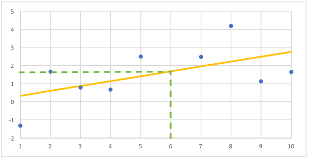
In ML terminology, the best fit line is called the model (or representation). It is described by two numbers, the slope and intercept, which are called its parameters. The job of the learning algorithm is to find the values of the model parameters that will work best for predicting new examples. Choosing these parameters is called training or fitting the model. Linear regression is an algorithm for fitting this type of linear model.
As noted above, our goal in supervised learning is to accurately predict the labels of new examples. This is the critical difference compared to the usual setting for linear regression. In the latter, we normally judge the quality of the model with its R2, which is only a measure of how well the model fits the given examples.
An implicit assumption, when using linear regression for prediction, is that a better fit on the given examples will translate into better predictions on new examples. For linear models, this is sometimes true. A (nearly) straight line in the given examples is strong evidence of a true relationship between the features and label that will hold up on new examples because straight lines rarely occur accidentally in nature. On the other hand, weak correlations, of say 10-20%, do not seem to be rare and those relationships frequently do not continue to hold on new examples.
ML models typically have far more parameters than this — often so many that it becomes easy to fit them almost perfectly to any set of examples you give them. As a result, the quality of the fit on the given examples does not have a simple relationship with accuracy on new examples. In fact, it is normal to find that tuning the parameters to match the given examples too closely actually worsens accuracy on new examples! This is called overfitting.
How then can we estimate the accuracy of our model if we can't just look at the fit on the given examples? The standard approach in ML is to do an experiment. First, randomly split the data into, for example, 80% training data and 20% test data. Fit the model using only the training data, and then test it using only the test data. The error rate of the model on the test data is a good estimate of the error rate on new examples. With this approach, our only implicit assumption is the unavoidable one that new examples are similar to the given ones. (Learning is impossible in principle if that does not hold.)
In summary, since linear regression is itself a machine learning algorithm, moving from a statistical to a machine learning setting is largely just learning new terminology. However, there is one key change that we must make in our process in order to use machine learning methods:
Measure the quality of the model by its performance on separate examples — not the ones used to fit the model.
As the earlier examples noted, this process change may be beneficial even when using linear regression.
Speaking of terminology, there are additional terms that we will need below. In the cases described above, we wanted a way to predict a number that can take on a wide range of possible values: the Ys in the table above range from 54 to 101, with any number in between being a reasonable prediction. In other cases, however, we want to predict a value that can only take on a small number of values. In particular, we might want to predict a value that can be only 1 or 0, indicating, for example, success or failure. The latter type of supervised learning problem is called classification, in contrast to the regression problems we considered above.
In general, machine learning algorithms designed for regression problems have versions that work for classification problems and vice versa. For example, we can replace linear regression with logistic regression, another standard statistical tool, to solve classification problems. While there may be reason to formulate a particular problem of interest as one rather than the other, we will treat classification and regression similarly and switch between them as best fits the situation.
Boosted Decision Stumps
One of the (very few) general ideas in machine learning that can be applied to almost any machine learning problem to improve results is the following: use ensembles, not individual models. That is, if you have a few different models that each work reasonably well on their own, combining them all together — say, by averaging their predictions — will usually work even better. You can think of this as a wisdom-of-the-crowd effect.
The Netflix prize was a famous example of this. Both the winning algorithm and the runner-up were ensembles of over a hundred different models. When those two were combined together, the results improved even further.
Boosted decision stumps take this idea to an extreme. They use a severely limited type of model — even simpler than linear regression — called a decision stump. Each stump asks a yes/no question about one feature of the input and then makes a guess based on that answer alone. For example, here is a stump that guesses someone's gender based solely on whether their height is above 5' 7" or not:
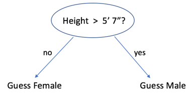
An individual stump like this will usually be a very poor predictor of the label. However, as we will see, by combining many stumps, we can produce an ensemble model that is more accurate than linear regression.
Boosting
I will describe boosting in the classification setting, where our goal is to predict a label of 1 or 0, success or failure. The regression version differs in some details but is broadly similar.
Rather than building a collection of independent models and then averaging their predictions, as suggested above, boosting works by building a sequence of models, where each is dependent on the ones built before. Specifically, each new model is built to try to fix the mistakes made by the previous model.
The process starts by building the first model using all of the training data. Then it builds the next model, also using all the training data but with extra "weight" placed on the examples that the first model got wrong. For the third model, more weight is added to the examples missed by the second model, and so on. This process can continue until the ensemble contains upwards of 50 or 100 individual models.
Adding weight to certain examples means increasing the importance that the training algorithm places on getting them right. This is easy to do, for any algorithm, if we want to, for instance, double the importance of a subset of the examples. In that case, we just need to add a second copy of each of those examples. Now, when the algorithm tallies up the mistakes, any errors in these particular examples will be doubled.
Without getting into the mathematics of it, it turns out to be similarly easy, with almost any machine learning algorithm, to increase the weight on an example by a fractional amount (e.g., by 14%) if we so choose. The boosting algorithm uses this flexibility to increase the weights of the mistakes by the exact percentage that makes the total weight of all examples with the mistakes equal to the total weight of the examples with correct predictions. In other words, it builds the next model using a set of weighted examples where the previous model would have a weighted-average accuracy of 50% — no better than random guessing.
That completes the description of how the ensemble is built. However, we still have to decide how to make predictions on new examples using the ensemble.
One option would be to let each individual model vote for its prediction and then let the overall model take whichever prediction gets a majority of votes. Boosting improves upon this by considering the accuracy of the individual models. Without getting into the details, a simple majority vote is replaced with a weighted-majority vote, where each model's weight is a function of its accuracy on the weighted set of examples on which it was trained. That is, models that were more accurate on the weighted training examples get more weight in the vote than those that were less accurate.
While we still need to discuss how to build the individual models, this completes the description of the AdaBoost algorithm for building and applying an ensemble of models. This approach, particularly when used with types of decision tree models, like the decision stumps we will study next, has been called the best "off the shelf" ML algorithm. While no ML algorithm works best for all problems, boosting gives good results for a broad range of problems and (at least at one time) state-of-the-art results for several important uses like click prediction on search results or ads.
Decision Stumps
The power of ensembling is such that we can still build powerful ensemble models even when the individual models in the ensembles are extremely simple. We will take advantage of this by making our individual models be decision stumps, nearly the simplest models you could imagine.
The simplest model we could construct would just guess the same label for every new example, no matter what it looked like. The accuracy of such a model would be best if we guess whichever answer, 1 or 0, is most common in the data. If, for instance, 60% of the examples are 1s, then we'll get 60% accuracy just by guessing 1 every time.
Decision stumps improve upon this by splitting the examples into two subsets based on the value of one feature. Each stump chooses a feature, say X2, and a threshold, T, and then splits the examples into the two groups on either side of the threshold. For each of these subsets, we still use the simplest model — just guessing the most common value within the subset — but we now give different answers for the two sides.
To find the decision stump that best fits the examples, we can try every feature of the input along with every possible threshold and see which one gives the best accuracy. While it naively seems like there are an infinite number of choices for the threshold, two different thresholds are only meaningfully different if they put some examples on different sides of the split. To try every possibility, we can sort the examples by the feature in question and try one threshold falling between each adjacent pair of examples.
The algorithm just described can be improved further, but even this simple version is extremely fast in comparison to other ML algorithms (e.g., training neural networks).
To see this algorithm in action, let's consider a problem that NFL general managers need to solve: predicting how college wide receivers will do in the NFL. We can approach this as a supervised learning problem by using past players as examples. Below are examples of receivers drafted in 2014. Each one includes some information known about them at the time along with their average receiving yards per game in the NFL from 2014 to 2016:
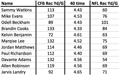
Any application of these techniques to wide receivers would try to predict NFL performance from a number of factors including, at the very least, some measure of the player's athleticism and some measure of their college performance. Here, I've simplified to just one of each: their time in the 40-yard dash (one measure of athleticism) and their receiving yards per game in college.
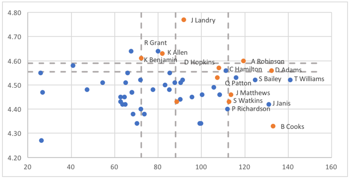
We can address this as a regression problem, as in the table above, or we can rephrase it as classification by labeling each example as a success (1, orange) or failure (0, blue), based on their NFL production. Here is what the latter looks like after expanding our examples to include players drafted in 2015 as well:
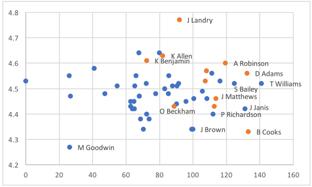
The X-axis shows each player's college receiving yards per game and the Y-axis shows their 40-time. One benefit of switching to classification is that we can easily visualize these data in two dimensions rather than three.
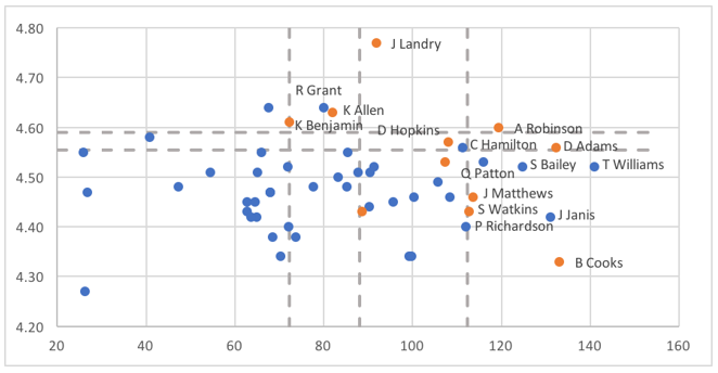
Returning to our boosting algorithm, recall that each individual model in the ensemble votes on an example based on whether it lies above or below the model's threshold for its feature. Here are what the splits look like when we apply AdaBoost and build an ensemble of decision stumps on these data:
The overall ensemble includes five stumps, whose thresholds are shown as dashed lines. Two of the stumps look at the 40-yard dash (vertical axis), splitting at values between 4.55 and 4.60. The other three stumps look at receiving yards per game in college. Here, the thresholds fall around 70, 90, and 110.
On each side of the split, the stumps will vote with the majority of the examples on that side. For the horizontal lines, there are more successes than failures above the lines and more failures than successes below the lines, so examples with 40-yard dash times falling above these lines will receive yes votes from those stumps, while those below the lines get no votes. For the vertical lines, there are more successes than failures to the right of the lines and more failures than successes to the left, so examples get yes votes from each of the stumps where they fall to the right of the line.
While the ensemble model takes a weighted average of these votes, we aren't too far off in this case if we imagine the stumps having equal weight. In that case, we would need to get at least 3 out of 5 votes to get the majority needed for a success vote from the ensemble. More specifically, the ensemble predicts success for examples that are above or to the right of at least 3 lines. The result looks like this:
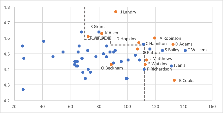
As you can see, this simple model captures the broad shape of where successes appear (and in a non-linear way). It has a handful of false positives, while the only false negative is Odell Beckham Jr., an obvious outlier. As we will see with some investing examples later in the article, the ability to adjust for non-linear relationships between features and outcomes may represent a key advantage over the traditional linear regression used in many investing factor models.
Visualizing Ensembles of Decision Stumps
If we have more than two features, it becomes difficult to visualize the complete ensemble the way we did in the picture above. (It is sometimes said that ML would not be necessary if humans could see in high dimensions.) However, even when there are many features, we can still understand an ensemble of decision stumps by analyzing how it views each individual feature.
To see how, let's look again at the picture of all the stumps included in the ensemble:
As we see here, there are two stumps that decide based on the 40-yard dash time. If an example has a 40-yard dash time above 4.59, then it receives a success vote from both of these stumps. If it has a time below 4.55, then it receives a no vote from both. Finally, if it fails between 4.55 and 4.59, then it receives a success vote from one stump but not the other. The overall picture looks like the following.
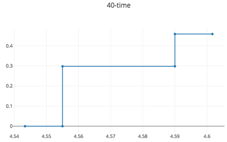
This picture accounts for the fact that the ensemble is a weighted average of the stumps, not a simple majority vote. Those examples with 40-yard dash time above 4.55 get a success vote from the first stump, and that vote has a weight of 0.30. Those with a time above 4.59 get a success vote from the second stump as well, but that stump is only weighted at 0.16, bringing the total weight for a yes vote up to 0.46. As you view this picture and the next, keep in mind that, in order for the model to predict "success" for a new wide receiver, that player would need to accumulate a total weight of at least 0.5.
The picture for the other feature, college receiving yards per game, looks like this:
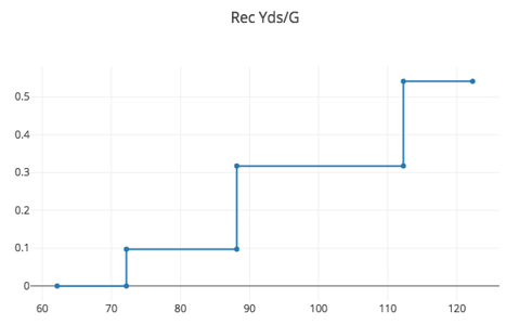
There are three stumps that look at this feature. The first, with a weight of 0.10, votes success on all examples with receiving yards per game at least 72 (or so). The next stump, weight a weight of 0.22, votes success on all examples above 88. Examples with yards above 88 receive success votes from both stumps, giving a weight of at least 0.32 (0.10 plus 0.22). The third stump adds an additional success vote, with weight of about 0.22 to examples with receiving yards per game above 112. This brings the total weight of the success votes for those in this range up to about 0.54.
Each of these pictures shows the total weight of success votes that an example will receive from the subset of the ensemble that uses that particular feature. If we group together the individual models into sub-ensembles based on the feature they examine, then the overall model is easily described in terms of these: the total weight of the success votes for an example is the sum of the weights from each sub-ensemble, and again if that total exceeds 0.5, then the ensemble predicts that the example is a success.
For classification problems with more features, while we cannot draw all the examples in a 2D plot with orange and blue dots as we did earlier, we can still draw pictures for the sub-ensembles using each feature. That gives us an easy way to visualize and understand ensembles of decision stumps.
Comparison with Linear Models
It will be worthwhile to compare these models to the linear models produced by linear or logistic regression.
An ensemble of decision stumps can be described with pictures of the weight of the success votes given according to each feature. Linear models instead give us just a single number for each feature. That number describes the slope of a line. For logistic regression, this line describes how much the odds of being a success vs a failure increases as the value of that feature increases. It is analogous to a picture like the ones we saw above but now a straight line like this:
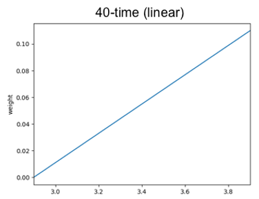
Just like an ensemble of decision stumps, the logistic regression model gets a weight by seeing where the example falls on the picture for each feature and then predicts success if the sum of those weights exceeds some value.
The key difference, though, is that the pictures used by logistic regression are restricted to being straight lines, whereas those from an ensemble of decision stumps can have more general shapes.
It is important to note that an ensemble of decision stumps can approximate a straight line as closely as it wants by adding enough stumps. Here is an example that approximates the line with 20 stumps:
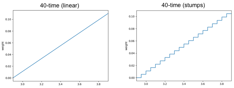
An ensemble of decision stumps has it within its power to approximate a straight line like this, but as we will see in the examples below, it usually chooses not to, instead finding that other shapes more accurately describe the data.
A linear model, in contrast, forces us to make predictions that scale linearly in each parameter. If the weight on some feature is positive, then increasing that feature predicts higher odds of success no matter how high it goes. The ensemble of stumps, which is not bound by that restriction, will not build a model of that shape unless it can find sufficient evidence in the data that this is true.
Ensembles of decision stumps generalize linear models, adding the ability to see non-linear relationships between the labels and individual features.
Application: Predicting Receivers From College to the NFL
To see a more realistic example of applying these techniques, we will expand upon the example considered above. Using only two features before made it easy to visualize the examples, but in practice, we want to include more information for improved accuracy.
We can start by adding age, which is useful because production at a younger age, when the player may be at a physical disadvantage, is a stronger signal than at an older age. (See JuJu Smith-Schuster for a recent example.) Next, we will expand our measures of athleticism from just the 40 time to also include the vertical jump and weight. Finally, we will add several additional measures of college production: absolute numbers of receptions, yards, and TDs per game, along with market shares of his team's totals of those. We will include those metrics from their final college season along with career totals. Altogether, that brings us to a total of 16 features.
Above, we looked at only two years of data. My full data set goes back to 2000, giving us 420 drafted wide receivers in total. This is still a tiny data set, by any measure, which gives linear models more of an advantage since the risks of overfitting are even larger than usual.
I randomly split the data into a training set and test set, with 80% in the former and 20% in the latter. Logistic regression mislabels only 13.7% of the training examples. This corresponds to a quite respectable "Pseudo R2" (the classification analogue of R2 for regression) of 0.29. However, on the test set, it mislabels 23.8% of the examples. This demonstrates that, even when using standard statistical techniques, in-sample error rate is not a good predictor of out-of-sample error.
The model produced by logistic regression has some expected parameter values: receivers are more likely to be successful if they are younger, faster, heavier, and catch more touchdowns. It does not give any weight to vertical jump. On the other hand, it still includes some head-scratching parameter values. For example, a larger market share of team receiving yards is good, but a larger absolute number of receiving yards per game is bad. (Perhaps interpretability problems are not unique to machine learning models!)
The ensemble of stumps model improves the error rate from 23.8% down to 22.6%. While this decrease seems small in the abstract, keep in mind that there are notable draft busts every year, even when decisions are made by NFL GMs who study these players full-time. My guess is that an error rate around 20% may be the absolute minimum that we could expect in this setting, so an improvement to 22.6% is no small achievement.
Like the logistic regression model, the ensemble of stumps likes wide receivers that are heavier and faster. However, it does not let these increase without bound. In particular, it does not distinguish between 40 times slower than 4.65, while the logistic regression model is forced to do so.
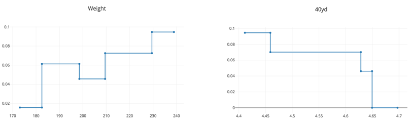
With the most important measures of college production, we see some clear non-linearity. While the model likes to see a market share of receiving yards and of receiving TDs that is high, it gives less of a bump to examples where these are too high. One hypothesis would be that those players are able to so dominate their team's production because they play on unique offenses with special roles that will not exist in the NFL.
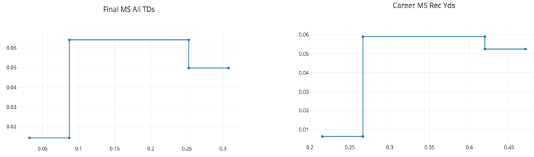
Interestingly, while the logistic regression model ignores vertical jump, the ensemble of stumps model includes that but instead ignores final season and career market shares of receiving TDs.
APPLICATION: PREDICTING RETURNS FROM COMPOSITE METRICS
For our last example, we switch from sports to finance. One of the most important uses of linear regression in the academic literature is to explain the cross section of returns in terms of factors. Let's see what this looks like using our non-linear ensemble of stumps model.
To do so, we will need to switch from classification back to regression. Our goal is to explain the 12-month return of an individual stock. Since return does not always take on one of a small set of values (e.g., just 0 or 1), this is a regression problem.
Stumps are easy to use for regression problems as well. As before, each stump compares the value of one feature to a threshold, but now, rather than guessing the most common label from the training data on that side of the threshold, we guess the average value.
Although I will skip the details here, our algorithm from above for learning an ensemble of stumps is also easily changed to work for regression instead.
For this example, our feature will be one of the OSAM composites that improves upon the traditional factors like "HML" for value. As many have demonstrated, we get more alpha in practice by combining multiple different metrics that try to capture the value effect rather than using a single metric like the P/B used to define HML.
We will look at all the stocks in a large cap universe (like the S&P 500). For each month going back to 1964, we rank all the stocks in the universe by composite score, and then turn that into a percentile between 1 and 100. Each stock in each month becomes an example with its percentile as the sole feature and its return as the label.
Fitting an ensemble of stumps to these data gives the following models for value and momentum:
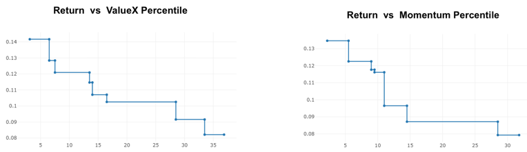
Rather than being strictly linear, both composites give a noticeably higher prediction only to the best 30–40% of all stocks by the metric and are flat for all higher percentiles. These plots cut off at that point (and the 40th to 100th percentiles are not shown) because higher percentiles all have the same prediction.
We also see non-linearity when looking at shareholder yield:
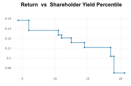
Here we see a much larger prediction for the best quintile of stocks, with the best 6% seeing an even higher prediction. Meanwhile, all the stocks falling in the 20th to 100th percentiles get the same prediction.
It is also possible to approach the problem we considered above using classification rather than regression. Instead of labeling each example with the return of the stock, we could instead label as successes those stocks that, say, end up in the top quintile of returns over that period, and then use a classifier to predict success.
Applying that to the Value composite, we might predict that the resulting ensemble of stumps classifier would give more weight to examples in precisely the same pattern as the ensemble of stumps regressor we saw above. However, we instead see a very different shape:
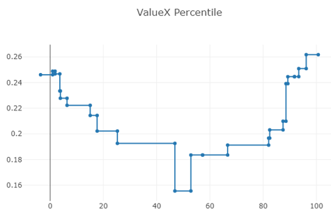
While the regressor continued to predict lower returns for increasing rank, here, the probability of being in the top quintile rebounds for the highest percentiles. That could be because such stocks are just more volatile than the others, giving them an increased chance of ending up in the top quintile by randomness alone. We also know that many of the most impressive returns come from stocks that are expensive — while the expensive group as a whole does poorly, many of the highest individual returns come from stocks that are pricey at the start of their run.
Conclusion
As these examples demonstrate, real-world data includes some patterns that are linear but also many that are not. Switching from linear regression to ensembles of decision stumps allows us to capture many of these non-linear relationships, which translates into better prediction accuracy for the problem of interest, whether that be finding the best wide receivers to draft or the best stocks to purchase.
If you want to test out these techniques on the data sets described above or apply them to your own data, I've put a simple implementation of these algorithms into a web page available here. If you have any questions or run into any problems, just hit me up on twitter, @kczat.
My hope is that you'll find the move from linear regression to ensemble of decision stumps to be an easy one. As we discussed above, the only change this requires in your process is to switch from measuring the accuracy of the model on the examples you used to train it (as is typical with R2) to measuring its accuracy on held-out data. That change not only allows you to use ensembles of decision stumps but, in fact, puts the entire spectrum of machine learning algorithms at your disposal. We will dive into some of the other ML algorithms that should interest you in future articles.