Appendix B: Mathematics of Return Decomposition

<< Return to Full Research Post: Factors from Scratch

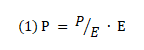
We can write the price P of a security as the product of its price-earnings multiple P/E and its earnings E: 

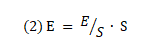
We can also write the earnings E of a security as the product of its profit margin E/S and its sales S. 

Combining (1) and (2), we get: 

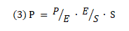
Equation (3) tells us that the price of security equals its price-earnings multiple times its profit margin times its sales. 

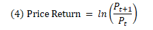
Now, we can define a security’s price return over the period from time t to t+1 as the logarithmic of the ratio of its price at t+1 to its price at t: 

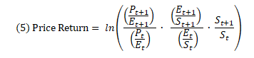
Substituting (3) into (4) we get: 

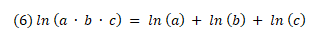
Now, mathematically, a logarithm of a product of terms equals the sum of the logarithms of each term. 

We can therefore write the price return as:

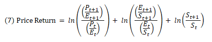
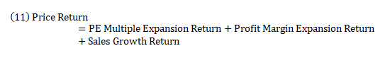
Each of the logarithmic terms in (7) represents a contribution from a different source of return. 

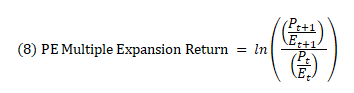
The first is multiple expansion. We define the return from multiple expansion as: 

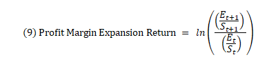
The second source is margin expansion. We define the return from margin expansion as: 

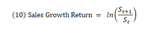
The third source is sales growth. We define the return from sales growth as: 

Combining (7), (8), (9), and (10), we arrive at the following conceptual equation for the decomposition of the price return: 

If we want, we can substitute the earnings growth return for the sum of margin expansion return and sales growth return: 

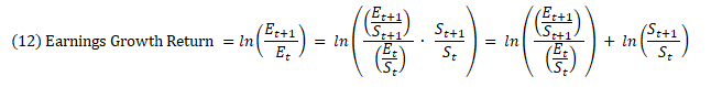
We then get: 

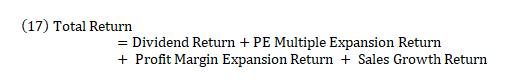
Now, if the security pays dividends, then to get to the total return we have to add the return from the dividends to the price return. With TR denoting the total return index of the security, we define the Total Return and the Dividend Return as follows:

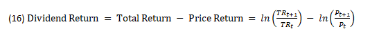
Substituting (15) and (16) into (11), we arrive at a final equation for decomposition: 

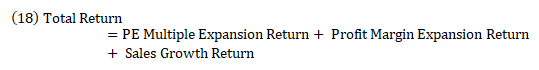
Now, our index construction methodology converts all dividends into share buybacks spread across the index. The price return therefore becomes equal to the total return, and the dividend return term goes away: 

We’ve written this equation in terms of earnings and sales, but we could have written it using a myriad of other fundamental metrics—EBITDA, Cash Flow, Book Value, and so on. The only constraint is that the mathematical relationships between the metrics have to work out in an analogous way. 

Now, the terms on the right side of equation (18) are logarithmic terms whose numeric values are not intuitively recognizable. To make those values more intuitively recognizable, we convert them to annual percent changes. We carry out the conversion by calculating the fractional logarithmic return contributions of each source, and then scale those individual contributions to the total return expressed as an annual percent change number. The previous sentence is likely to be somewhat confusing, so we illustrate below with an example.

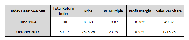
Suppose that we want to decompose the returns of the S&P 500 from June of 1964 to October of 2017 using the following index data: 

Applying the above equations, we calculate the different logarithmic returns of each source and the association fractional contribution of each source to the total logarithmic return: 

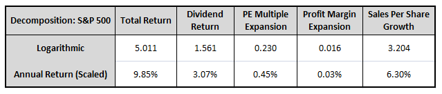
Sales growth, for example, contributed a logarithmic return of 3.204, relative to a logarithmic total return of 5.011. Its fractional contribution to the total was therefore 3.204/5.011 = 63.94%. What this means is that, logarithmically, 63.94% of the index’s total return came from sales growth. To convert the 3.204 logarithmic sales growth number into an annual percent change number, we multiply the fractional contribution of 63.94% times the annual total return for the index, which was 9.85%. We get 6.30%, which we refer to as the annual return contribution from sales growth. 

Applying this technique to all the return sources, we conclude that dividends, PE multiple expansion, profit margin expansion, and sales growth added returns of 3.07%, 0.45%, 0.03%, and 6.30%, which adds up to a 9.85% total return. Admittedly, this way of speaking is not mathematically meaningful. The only return numbers that properly add up in that way are logarithm returns. We use the scaling approach simply as a heuristic to make the numbers more intuitive and recognizable to investors. Because the numbers are scaled to the total return in the correct logarithmic proportions, they convey the underlying return contribution information in a way that is accurate. 

<< Return to Full Research Post: Factors from Scratch